Introduction

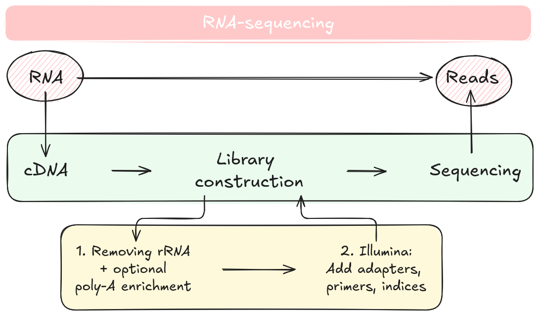
RNA-seq is a leading method for quantifying RNA levels in biological samples, leveraging next-generation sequencing (NGS) technologies. The process begins with RNA extraction and conversion to cDNA, followed by sequencing to produce reads representing the RNA present in a sample.

RNA-seq overview

Lab Protocol Overview

RNA-seq data (i.e. reads) are processed through a standard workflow with three main stages:

1. Data pre-processing – improves read quality by removing contaminants and adapters.
2. Alignment and quantification – maps reads to a reference genome and estimates gene expression, either through traditional or faster lightweight methods.
3. Differential expression analysis – identifies and visualizes genes with significant expression differences.

Additional downstream analyses (e.g., functional enrichment, co-expression, or multi-omics integration) are popular ways to derive biological insights from these analyses.

Adapted from: https://nf-co.re/rnaseq/dev/docs/usage/differential_expression_analysis/theory

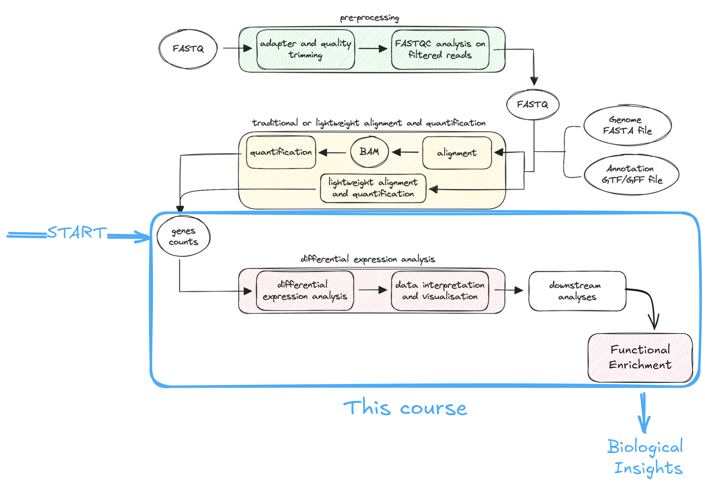
Note | As shown in the above scheme, this course will not cover the first two steps. It will begin with a gene count matrix and proceed with differential expression analysis, visualization, and a brief overview of functional enrichment.

Differential expression

Differential expression (DE) analysis compares gene expression levels across conditions (e.g., disease vs. healthy) to identify genes with statistically significant changes. This is typically done using tools like DESeq2, a robust R package designed for analyzing RNA-seq count data.

1. Input Requirements:

   • A count matrix (genes × samples).
   • A metadata table describing sample attributes.

2. Quality Control:

   • Use PCA and hierarchical clustering to explore variation and detect outliers.
   • Transform counts using variance stabilizing transformation (vst) or regularized log (rlog) to ensure comparable variance across genes, improving downstream analysis.

3. Filtering:

   • Remove genes with low or zero counts to improve sensitivity and reduce false positives.

4. Design Formula:

   • Specifies how gene counts depend on experimental factors.

   • Can include main conditions and covariates (e.g., gender, batch, stage).

   • Example:

     design = ~ condition
     design = ~ gender + developmental_stage + condition

   • The main factor of interest is usually placed last for clarity.

DE with DESeq2

DESeq2 is a widely used R package for identifying differentially expressed (DE) genes from RNA-seq count data. RNA-seq data typically exhibit many low-count genes and a long-tailed distribution due to highly expressed genes, requiring specialized statistical modeling. The major steps in DESeq2 are the following:

1. Normalization

   • Adjusts for sequencing depth and RNA composition using size factors calculated via the median ratio method.
   • Normalized counts are used for visualization but raw counts must be used for DESeq2 modeling.

2. Dispersion Estimation

   • RNA-seq data show overdispersion (variance > mean).

   • DESeq2 models count data using the negative binomial distribution.

   • Dispersion is estimated:

     • Globally (common dispersion),
     • Per gene (gene-wise dispersion),
     • Then refined through shrinkage toward a fitted mean-dispersion curve to improve stability, especially with small sample sizes.

   • Genes with extreme variability are not shrunk to avoid false positives.

3. Model Fitting and Hypothesis Testing

   • A generalized linear model (GLM) is fit to each gene’s normalized counts.

   • DESeq2 tests whether gene expression differs significantly between groups:

     • Wald test for simple comparisons (e.g., treated vs. control),
     • Likelihood Ratio Test (LRT) for more complex designs with multiple variables.

   • Each test returns a log2 fold change and a p-value.

4. Multiple Testing Correction

   • To control for false positives from testing thousands of genes, DESeq2 adjusts p-values using Benjamini-Hochberg FDR correction.
   • An FDR cutoff of <0.05 means that 5% of DE genes may be false positives.

Functional analysis

After identifying differentially expressed (DE) genes, functional analysis helps interpret their biological relevance by uncovering the pathways, processes, or interactions they may be involved in. This includes:

• Functional enrichment analysis – identifies overrepresented biological processes, molecular functions, cellular components, or pathways.
• Network analysis – groups genes with similar expression patterns to reveal potential interactions.

This course focuses on Over-Representation Analysis (ORA), a common enrichment method that uses the hypergeometric test to assess whether certain biological pathways or gene sets are statistically enriched in the DE gene list.

Key components of ORA:

• Universe – the full set of genes considered (e.g., all genes in the genome).
• Gene Set – a group of genes annotated to a particular function or pathway (e.g., from Gene Ontology).
• Gene List – the list of DE genes identified in the analysis.

The test evaluates whether the overlap between the DE gene list and a gene set exceeds what would be expected by chance, pointing to potentially meaningful biological mechanisms.

Tools commonly used for functional enrichment include Gene Ontology, KEGG, Reactome, clusterProfiler, and g:Profiler. These support the biological interpretation of DE results and help uncover pathways affected by the experimental condition.

---