Topic 2 | Introduction to R

Class Details

📅 Date: March, 2026
📖 Synopsis: Brief introduction to R

R Intro

First, we will discuss the purpose of learning to program in R.
Then, you will be introduced on how to install and use R and RStudio.
Next, you will follow an interactive learning tutorial, self-paced, using the swirl package.
Finally, you will recap some important notes about R programming.

Questions to debate in class:

Why do we need to use computer programming?
Why do we use R?
Are there other alternatives to R?

Learning R: Tutorials and Mini-projects

1. Using RStudio

The practical classes for this course require R and RStudio.

Please read the General information tab to get information on how to use your RStudio Server account from the virtual machines at UAlg (provided by the instructor), or how to install R and RStudio in your system.

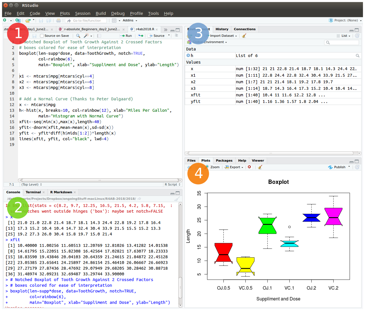
The friendliest way to learn R is to use RStudio which is an Integrated Development Environment - IDE - that includes:

a text editor with syntax-highlighting (where you save the R code in a script to run again in the future);
an R console to execute code (where the R instructions are executed and evaluated to generate the output);
a workspace and history management;
and tabs to visualize plots and exporting images, browsing the files in the workspace, managing packages, getting help with functions and packages, and viewing html/pdf or presentation files created within RStudio (using RMarkdown).

Figure 1: RStudio Graphical User Interface (GUI)

**2. Load the swirl package & Follow the guided course**

After you become familiarized with RStudio, we shall progress to the interactive, self-paced, hands-on tutorial provided by the swirl package. You will learn R inside R. For more info about this package, visit: https://swirlstats.com/

Type these instructions in the R console (panel number 2 of RStudio). The words after a # sign are called comments, and are not interpreted by R, so you do not need to copy them.
You can copy-paste the code, and press enter after each command.

install.packages("swirl")   # Install swirl (once if not installed)

library("swirl")            # Load the swirl package to make it available for you to use
swirl()                     # Start swirl

After starting swirl, follow the instructions given by the program, and complete all of the following lessons:

Please install the course:
1: R Programming: The basics of programming in R

Choose the course:
1: R Programming

Complete the following lessons, in this order:
1: Basic Building Blocks
3: Sequences of Numbers
4: Vectors
5: Missing Values
6: Subsetting Vectors
7: Matrices and Data Frames
8: Logic
12: Looking at Data
15: Base Graphics

Please call the instructor for any question, or if you require help.
Now, just Keep Calm… and Good Work!

If you already have some knowledge of R, but need to refresh your memory, your are in the right place!

Hands-on Tutorial

Welcome

Learning a programming language is much like learning a spoken language: you need to understand the grammar before you can write good sentences, and fluency comes with practice. R is no different. This tutorial introduces you to the foundational concepts of R one step at a time, building each new idea on the previous one.

By the end of this tutorial you will be comfortable with:

Setting up a reproducible working environment in RStudio
Understanding R’s core syntax and operators
Working with R’s five fundamental data structures
Controlling the flow of a program with loops and conditionals
Writing your own functions
Loading data from files and saving results
Using a selection of R’s most useful built-in functions

Note

This tutorial assumes you have used R before at a basic level - you know what a variable is and have run at least a few commands. If you have never opened R or RStudio, go to the learn R tab first, and follow the swirl course.

Setting up Your Workspace

RStudio as Your R Environment

RStudio is an Integrated Development Environment (IDE) built specifically for R. It organises your work into four panes:

Source editor - where you write and save R scripts.
Console - where R executes commands and shows output.
Environment / History - shows all objects currently in memory and your command history.
Files / Plots / Packages / Help - a multi-purpose panel for browsing files, viewing plots, managing packages, and reading documentation.

You will spend most of your time in the source editor and the console.

Creating an RStudio Project

Projects are one of the most useful features in RStudio. They keep all files related to an analysis - data, scripts, and outputs - in one self-contained folder, and they automatically set that folder as your working directory whenever you open the project.

To create a new project:

File > New Project... > New Directory > New Project
Directory name:  r_tutorial
Create project as subdirectory of:  ~/   (or wherever you prefer)
Create Project

Once created, open the project options in the upper-right corner of RStudio and set the following in R General:

Restore .RData at startup   ->  No
Save .RData on exit         ->  Ask
Always save history         ->  Yes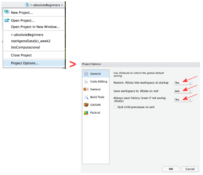

Setting “Restore .RData” to No is important: it forces your scripts to be self-contained and reproducible, rather than relying on objects left over from a previous session.

Your Working Directory

The working directory is the folder R treats as its “home base” - it is where R looks for files you want to load, and where it saves files you write. Since you are using a project, this is already set for you, but these commands are useful to know:

getwd()        # print the current working directory path
dir()          # list all files in the working directory
setwd("~/r_tutorial")  # manually set the working directory (rarely needed with projects)

Saving and Quitting

R automatically tracks everything you type in .Rhistory, and can save all objects in memory to .RData. When you quit RStudio (via q() or the window close button), it will ask whether to save the workspace:

q()
# Save workspace image to ~/path/to/project/.RData? [y/n/c]:

For day-to-day work, it is usually better to answer no and rely on your script to recreate everything. The .RData file is mainly valuable when a computation takes a very long time and you want to preserve the result.

Tip

Get into the habit of writing your analysis in a script from the start - not just typing in the console. A good script is your analysis: it documents every step and lets you re-run everything from scratch at any time.

Packages: Extending What R Can Do

What Is a Package?

Base R is powerful, but its real strength comes from its ecosystem of packages - collections of functions, data, and documentation contributed by the R community. There are currently (in March 2026):

23,291 packages on CRAN, the main general-purpose repository.
2,361 packages on Bioconductor, focused on bioinformatics and genomics.

Installing and Loading Packages

You install a package once (it is saved to your computer), and load it at the start of each session (it is read into memory):

# Install a package from CRAN (only needs to be done once)
install.packages("ggplot2")

# Load the package so its functions are available in this session
library(ggplot2)

# You can also use a single function without loading the whole package
ggplot2::qplot(1:10, 1:10)

Other installation sources and their functions:

Source	Function
CRAN	`install.packages("pkg")`
Bioconductor	`BiocManager::install("pkg")`
GitHub	`remotes::install_github("u/pkg")`
Any of above	`pak::pkg_install("pkg")`

Getting Help

R has thorough built-in documentation. Learning to use it is one of the best investments you can make early on:

?mean                    # help page for a specific function
help(mean)               # same as above
help(package = "ggplot2")  # overview of an entire package
vignette("ggplot2")      # longer worked examples (called vignettes)

Tip

When you encounter a function you do not recognise, your first instinct should be ?function_name. The Examples section at the bottom of each help page is usually the fastest way to understand what a function does.

Operators

Operators are the building blocks of R expressions. Before working with complex data structures, you need to understand how R evaluates expressions.

Arithmetic Operators

R works as a very capable calculator:

Operator	Meaning	Example	Result
`+`	Addition	`3 + 4`	`7`
`-`	Subtraction	`10 - 3`	`7`
`*`	Multiplication	`3 * 4`	`12`
`/`	Division	`7 / 2`	`3.5`
`^`	Exponentiation	`2 ^ 8`	`256`

Assignment Operators

In R, you store values in named objects using the assignment operator <-. Think of it as the arrow pointing a value into a container you are labelling:

x <- 7      # store the number 7 in an object called x
x           # typing the name prints its value

y <- 9
z <- 3

42 -> lue   # right-pointing arrow: value goes to the right
x ->  xx    # x (which holds 7) is copied into xx

my_variable <- 5

Note

You will also see = used for assignment. It works in most situations, but <- is the conventional R style and is unambiguous. This tutorial uses <- throughout.

Comparison Operators

These compare two values and always return TRUE or FALSE:

Operator	Meaning
`==`	Equal to
`!=`	Not equal to
`<`	Less than
`>`	Greater than
`<=`	Less than or equal
`>=`	Greater than or equal

1 == 1           # TRUE
1 != 1           # FALSE
x > 3            # TRUE  (x is 7)
y <= 9           # TRUE  (y is 9)
my_variable < z  # FALSE (5 is not less than 3)

Logical Operators

Logical operators combine TRUE/FALSE values:

Operator	Meaning
`&`	AND (vectorised - checks every element)
`&&`	AND (checks only the first element)
`\|`	OR (vectorised)
`\|\|`	OR (checks only the first element)
`!`	NOT (negation)

# AND: both conditions must be TRUE
7 < 9 & 7 > 10    # 7 < 9 is TRUE, but 7 > 10 is FALSE -> result is FALSE

# OR: at least one condition must be TRUE
7 < 9 | 7 > 10    # 7 < 9 is TRUE -> therefore the result is TRUE even if 7 > 10 is FALSE

# NOT inverts the result
!(x != y & my_variable <= y)   # x is 7; y is 9; my_variable is 3

Work through each expression carefully. The ability to combine conditions is essential for filtering data later.

The Pipe Operator

The pipe |> passes the result of one expression as the first argument to the next. It makes a chain of operations much easier to read:

# Without the pipe: you read from the inside out
round(sqrt(mean(c(5, 10, 15))), digits = 2)

# With the pipe: you read left to right
c(5, 10, 15) |> mean() |> sqrt() |> round(digits = 2)

Both produce the same result. The pipe version reads like a sentence: “take this vector, compute its mean, take the square root, then round to 2 decimal places.”

Note

The native pipe |> was introduced in R 4.1. You may also encounter %>% from the magrittr package, which works similarly. This tutorial uses |>.

R’s Five Core Data Structures

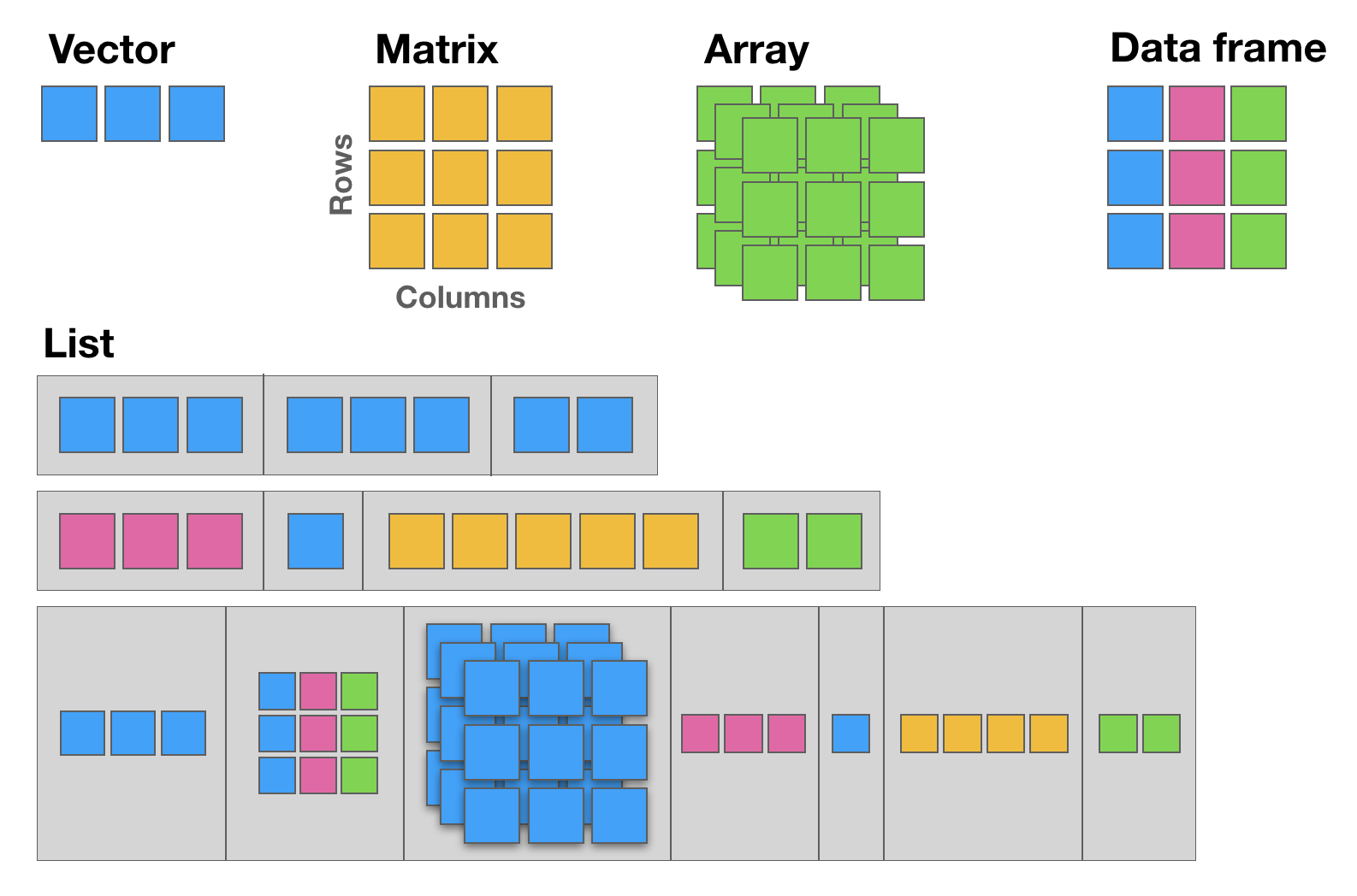
Everything in R is an object, and objects have a type (what they store) and a structure (how they are organised). The five structures below cover almost everything you will need:

Structure	Dimensions	Same data type?	Typical use
Vector	1D	Yes	A column of numbers or text
Matrix	2D	Yes	Numerical grids, linear algebra
Array	n-D	Yes	Multi-dimensional numerical data
Data frame	2D	No (yes by column)	Tabular datasets
List	Any	No	Mixed, nested objects
Factor*	1D	Yes (levels)	Categorical variables

*Factors are a class built on integer vectors, not a distinct data structure. They are included here because their behaviour differs meaningfully from plain vectors in modelling and plotting contexts.

Vectors

A vector is the fundamental building block of R. Every scalar value (a single number or string) is actually a vector of length one.

Creating vectors:

# c() combines values into a vector
x <- c(1, 2, 3, 4, 5, 6)
x
class(x)   # "numeric"

y <- "a string"
class(y)   # "character"

# Sequences
seq(1, 6)                        # 1 2 3 4 5 6
seq(from = 100, by = 1, length = 5)  # 100 101 102 103 104
1:6                              # shorthand for seq(1, 6)
10:1                             # counts backwards

# Repetition
rep(1:2, times = 3)   # 1 2 1 2 1 2
rep(1:2, each = 3)    # 1 1 1 2 2 2  (different behaviour -- try it)

Vectorised arithmetic:

One of R’s greatest strengths is that operations apply to all elements of a vector simultaneously - no loops needed:

1:3 + 10:12   # element-wise: 11 13 15

x <- c(1, 2, 3, 4, 5, 6)
x + 10        # 10 is recycled to match x's length: 11 12 13 14 15 16
c(70, 80) + x # 70 80 are recycled: 71 82 73 84 75 86

Warning

When vectors of different lengths are combined, R recycles the shorter one. If the longer vector’s length is not a multiple of the shorter one’s length, R completes the operation but also prints a warning. The warning is not an error - the result is still returned - but it signals that the recycling may not be intentional.

Subsetting vectors:

You extract elements from a vector using square brackets []. R uses 1-based indexing (this means that the first element is at position 1, not 0):

myVec <- 1:26
myVec[1]      # first element
myVec[6:9]    # elements 6 through 9

# LETTERS is a built-in vector of the 26 uppercase letters
myUni <- LETTERS
myUni[c(21, 1, 12, 7)]   # U A L G

# Logical subsetting: extract only elements where the condition is TRUE
myLogical <- myVec > 10
myVec[myLogical]   # returns 11 through 26

# More compactly (same result)
myVec[myVec > 10]

Naming vector elements:

joe <- c(24, 1.70)
names(joe) <- c("age", "height")
joe["age"] == joe[1]   # TRUE (both refer to the same element)

names(myVec) <- LETTERS
myVec[c("A", "A", "B", "C", "E", "H", "M")]   # The Fibonacci series

Excluding elements with -:

alphabet <- LETTERS
vowel_positions <- c(1, 5, 9, 15, 21)
alphabet[vowel_positions]    # the vowels

consonants <- alphabet[-vowel_positions]  # everything except the vowels
consonants

Matrices

A matrix is a two-dimensional vector: it has rows and columns but, like a vector, all elements must be the same type.

Note

R stores matrices in column-major order: it fills column 1 first, then column 2, and so on. This is the default (byrow = FALSE). Set byrow = TRUE to fill row by row instead.

my_matrix <- matrix(1:12, nrow = 3, byrow = FALSE)
dim(my_matrix)   # 3 rows, 4 columns
my_matrix

xx <- matrix(1:12, nrow = 3, byrow = TRUE)
xx   # compare with my_matrix to see the difference

Subsetting matrices:

Matrices use two-dimensional indexing: [row, column]. Leaving either blank means “all”:

my_matrix <- matrix(LETTERS, nrow = 4, byrow = TRUE)

my_matrix[, 2]          # all rows, column 2 (returns a vector)
my_matrix[3, ]          # row 3, all columns (returns a vector)
my_matrix[1:3, c(4, 2)] # rows 1-3, columns 4 and 2 (in that order)

Arrays

An array is essentially the generalisation of a matrix to any number of dimensions. A matrix is just a 2D array, and a vector is a 1D array - so the three form a natural hierarchy. In practice you encounter arrays most often in image analysis (height × width × colour channel), genomics (genes × samples × time points), and any situation where data naturally lives in a cube or hypercube rather than a flat table.

Data Frames

Data frames are the workhorse of data analysis in R. Think of them as spreadsheets: rows are observations, columns are variables. Unlike matrices, each column can be a different type - one column can hold numbers while another holds text.

df <- data.frame(
  type = rep(c("case", "control"), c(2, 3)),
  time = rnorm(5)
)
class(df)  # "data.frame"
df

Subsetting data frames:

Data frames support the same [row, column] indexing as matrices, plus named access with $:

# The iris dataset is built in -- a classic for learning data manipulation
iris[, 3]               # all rows, column 3 (Petal.Length)
iris[1, ]               # first row, all columns
iris[1:9, c(3, 4, 1, 2)]  # rows 1-9, reordered columns

# Column access by name
iris$Species
iris[, "Sepal.Length"]

Tip

Prefer df$column_name for interactive exploration and df[, "column_name"] when writing functions - the latter is easier to generalise.

Lists

Lists are R’s most flexible data structure. Each element can be anything - a vector, a data frame, another list, or even a function:

lst <- list(a = 1:3, b = "hello", fn = sqrt)
lst

lst$fn(49)   # calls sqrt(49) -> 7

Single vs double brackets:

This is a nuance that trips up many beginners. Remember this rule:

lst[1] returns a list containing the first element.
lst[[1]] returns the element itself in its native type.

lst[1]       # a list of length 1
class(lst[1])   # "list"

lst[[1]]     # the vector 1:3 itself
class(lst[[1]])  # "integer"

lst$b        # same as lst[["b"]] -- returns the element, not a list

Think of [ ] as taking a slice of the list (the result is still a list), and [[ ]] as reaching inside and pulling out the contents.

Factors

A factor represents a categorical variable - one that takes a limited set of distinct values called levels. Factors look like character vectors but are stored as integers with labels, making them memory-efficient and ensuring that statistical models treat them correctly.

my_fdata <- c(1, 2, 2, 3, 1, 2, 3, 3, 1, 2, 3, 3, 1)

# Convert to factor
factor_data <- factor(my_fdata)
factor_data
levels(factor_data)   # "1" "2" "3"

# Add meaningful labels
labeled_data <- factor(my_fdata, labels = c("I", "II", "III"))
labeled_data
levels(labeled_data)  # "I" "II" "III"

Note

Factors matter in modelling: R uses them to set up treatment contrasts automatically. If your categorical variable is stored as a plain character vector, functions like lm() still convert it internally, but controlling the levels and their order requires explicit factors.

Converting Between Data Structures

Sometimes you receive data in one structure but need it in another. R provides a family of as.*() functions for this:

class(lst)   # inspect the type of an object
str(lst)     # compact summary of any object's structure

as.matrix(df)         # data frame -> matrix (all columns coerced to same type)
as.data.frame(my_matrix)  # matrix -> data frame
as.numeric("3.14")    # character -> number
as.character(42)      # number -> character

Warning

Converting a data frame with mixed types to a matrix forces all columns to the same type. A data frame with numeric and character columns will become an all-character matrix, since character is the “broader” type.

Control Flow: Loops and Conditionals

Until now, every command has been executed once, in order. Control flow lets you repeat actions and make decisions - the ingredients of real programs.

`for` Loops

A for loop repeats a block of code for each value in a sequence:

# Compute the first 12 terms of the Fibonacci sequence
fib <- c(1, 1)
for (i in 1:10) {
  next_val <- fib[i] + fib[i + 1]
  fib <- c(fib, next_val)
}
fib

The loop variable i takes each value in 1:10 in turn. On each iteration, the code inside { } runs with that value of i.

`while` Loops

A while loop keeps running as long as its condition is TRUE:

x <- 3
while (x < 9) {
  cat("Number", x, "is smaller than 9.\n")
  x <- x + 1
}
# Note: x is now 9, so the loop stopped

Warning

Always ensure that something inside a while loop will eventually make the condition FALSE. If the condition never becomes FALSE, the loop runs forever.

`if` / `else` Conditionals

Conditionals run a block of code only when a condition is TRUE:

x <- -5
if (x >= 0) {
  print("Non-negative number")
} else {
  print("Negative number")
}

You can chain conditions with else if:

x <- 0
if (x > 0) {
  print("Positive")
} else if (x < 0) {
  print("Negative")
} else {
  print("Zero")
}

Combining a for loop with an if statement lets you process each element differently:

x <- -5:5
for (i in seq_along(x)) {
  if (x[i] > 0) {
    print(x[i])
  } else {
    print("negative or zero")
  }
}

`ifelse()` - Vectorised Conditionals

The ifelse() function applies a condition element-wise across a vector, returning one value where the condition is TRUE and another where it is FALSE:

gender <- c(1, 1, 1, 2, 2, 1, 2, 1, 2, 1, 1, 1, 2, 2, 2, 2, 2)
ifelse(gender == 1, "F", "M")   # This reads: If gender equals 1, then F, else M.

This is far more efficient than looping over each element with a for loop.

The `apply()` Family of Functions

Loops work, but in R there is often a cleaner alternative: the apply family of functions.

These functions apply a given function repeatedly across the elements of a data structure (rows, columns, or list elements) and return the results in a convenient form. They tend to produce more readable code than explicit loops, and in some cases are faster.

The family has several members. The three you will use most often as a beginner are apply(), lapply(), and sapply().

Function	Input	Output	Typical use
`apply()`	Matrix / data frame	Vector or matrix	Summaries across rows or columns
`lapply()`	List or vector	List	Transform every element of a list
`sapply()`	List or vector	Vector, matrix, or list	Like `lapply()` with automatic simplification

Tip

Three more members of the family are worth knowing once you are comfortable with the three above. tapply() applies a function to subsets of a vector defined by a grouping factor (useful for group-wise summaries). mapply() is a multivariate version that applies a function to multiple vectors in parallel. vapply() works like sapply() but requires you to declare the expected output type, making it safer to use inside your own functions.

`apply()` - Over Rows or Columns of a Matrix or Data Frame

apply(X, MARGIN, FUN) applies a function FUN to either every row (MARGIN = 1) or every column (MARGIN = 2) of a matrix or data frame X:

m <- matrix(1:12, nrow = 3)
m

apply(m, 1, sum)   # sum of each row:    6 22 38 (try it and see)
apply(m, 2, sum)   # sum of each column: 6 15 24 33... (try it)

# Works equally well with the iris data frame (numeric columns only)
apply(iris[, 1:4], 2, mean)   # column means
apply(iris[, 1:4], 2, sd)     # column standard deviations

A useful memory aid: MARGIN = 1 collapses across columns to give one result per row; MARGIN = 2 collapses across rows to give one result per column.

Note

apply() always coerces a data frame to a matrix first. This is fine when all columns are numeric, but will silently convert everything to character if any column is not (i.e. the same behaviour as as.matrix() on a mixed data frame).

`lapply()` - Over a List, Always Returns a List

lapply(X, FUN) applies FUN to each element of list (or vector) X and returns the results as a list of the same length:

lst <- list(a = 1:5, b = c(2.1, 3.7, 0.4), c = 10:1)

lapply(lst, mean)    # mean of each element; result is a list
lapply(lst, length)  # length of each element; result is a list

The returned list is always the same length as the input, and each element corresponds to the result of applying FUN to the matching input element. Because the output is always a list, lapply() is the safe, predictable choice: it never surprises you with an unexpected output type.

`sapply()` is like `lapply()`, but Simplifies the Result

sapply() calls lapply() internally, then tries to simplify the result to a vector or matrix if possible:

sapply(lst, mean)    # returns a named numeric vector, not a list
sapply(lst, length)  # returns a named integer vector

When all results are scalars of the same type, sapply() collapses them into a named vector, which is usually what you want for interactive exploration. When results cannot be simplified (for example because each element is a vector of different length), sapply() falls back to returning a list, just like lapply().

Tip

A practical rule of thumb: use lapply() when writing functions or packages (predictable output type), and sapply() when exploring data interactively (convenient output). If sapply() behaves unexpectedly, switch to lapply() and inspect the raw list.

Comparison: Loop vs Apply

To make the equivalence concrete, here is the same computation written three ways:

# Compute the mean of each numeric column in iris using a for loop
result_loop <- numeric(4)
for (i in 1:4) {
  result_loop[i] <- mean(iris[, i])
}
names(result_loop) <- colnames(iris)[1:4]
result_loop

# Using apply
result_apply <- apply(iris[, 1:4], 2, mean)
result_apply

# Using colMeans (a specialised shortcut worth knowing)
colMeans(iris[, 1:4])

All three produce the same result. The apply version is more concise; colMeans() is even more so for this specific case.

Note

colSums(), rowSums(), colMeans(), and rowMeans() (included in the useful built-in functions section below) are specialised shortcuts for the most common apply-over-margins operations. They are faster than the equivalent apply() calls and more readable when the intent is simply summing or averaging rows or columns.

Writing Your Own Functions

As your scripts grow, you will find yourself repeating the same sequence of steps. The solution is to wrap those steps in a function - a reusable, named block of code.

Function Syntax

my_function <- function(argument1, argument2, ...) {
  # body: computation goes here
  result <- argument1 + argument2
  return(result)
}

The return() call specifies what the function produces. If you omit it, R returns the value of the last expression in the body.

A Worked Example

Let’s write a function that computes the mean of a numeric vector, to understand what R’s built-in mean() is actually doing:

my_average <- function(x) {
  total   <- sum(x)
  n       <- length(x)
  average <- total / n
  return(average)
}

my_data <- c(10, 20, 30)
my_average(my_data)   # 20
mean(my_data)         # 20 -- same result

Default Argument Values

Functions can have default values for arguments, which are used when the caller does not supply them:

greet <- function(name, greeting = "Hello") {
  cat(greeting, name, "\n")
}

greet("Alice")           # Hello Alice
greet("Alice", "Hi")     # Hi Alice

Tip

Functions should do one thing well. If a function is getting long or hard to describe in a single sentence, consider splitting it into smaller functions.

Loading Data and Saving Results

Real analyses begin by reading in data and end by writing out results.

Writing Data to Files

# Inspect the built-in esoph dataset
esoph
dim(esoph)
colnames(esoph)

# Save as comma-separated values
write.table(esoph, file = "esophData.csv", sep = ",", quote = FALSE, row.names = FALSE)

# Save as tab-separated values
write.table(esoph, file = "esophData.tab", sep = "\t", quote = FALSE, row.names = FALSE)

Reading Data from Files

# Read the tab-separated file back into R
my_data_tab <- read.table("esophData.tab", sep = "\t", header = TRUE)

# Read the CSV file
my_data_csv <- read.csv("esophData.csv", header = TRUE)

Note

To read or write files outside your working directory, provide the full path: read.csv("/home/user/data/my_file.csv").

On Windows, use forward slashes / or double backslashes \\ in paths - a single backslash \ is a special character in R strings.

Modern Alternatives

The readr package (part of the tidyverse) provides faster, more robust functions:

# install.packages("readr")
library(readr)

write_csv(esoph, "esophData.csv")
my_data <- read_csv("esophData.csv")

readr functions are generally faster, produce more informative messages, and never silently convert strings to factors.

A Tour of Useful Built-in Functions

This final section introduces a selection of functions you will reach for repeatedly. The iris and esoph built-in datasets are used throughout.

Exploring a Dataset

head(iris)        # first 6 rows
tail(iris)        # last 6 rows
dim(iris)         # number of rows and columns
str(iris)         # compact structural overview
summary(iris)     # descriptive statistics for each column
colnames(iris)    # column names

Descriptive Statistics

mean(iris[, 2])     # mean of the second column
sd(iris[, 2])       # standard deviation
var(iris[, 2])      # variance
median(iris[, 2])   # median

min(iris[, 1])      # minimum
max(iris[, 1])      # maximum
range(iris[, 1])    # minimum and maximum together

Counting, Grouping and Summarising

# unique() removes duplicates
unique(iris$Sepal.Length)
length(unique(iris$Sepal.Length))   # how many distinct values?

# table() counts occurrences
table(iris$Species)

# colSums, rowSums, colMeans, rowMeans operate on an entire matrix or data frame
colSums(iris[, 1:4])    # sum of each column
rowSums(iris[, 1:4])    # sum of each row
colMeans(iris[, 1:4])   # mean of each column
rowMeans(iris[, 1:4])   # mean of each row

# aggregate() computes group-level summaries
aggregate(iris[, 1:4], by = list(species = iris$Species), FUN = mean)

Filtering and Selecting

# subset() with conditions
subset(iris,
       Petal.Length >= 3 & Sepal.Length >= 6.5,
       select = c(Petal.Length, Sepal.Length, Species))

# %in% tests membership
month.name[month.name %in% c("May", "July", "September")]

Sorting and Ordering

sort(iris[1, 1:4])    # values in ascending order
order(iris[1, 1:4])   # indices that would sort the vector
rank(iris[1, 1:4])    # rank of each element
rev(LETTERS)          # reverse a vector

Logical Tests on Vectors

any(iris[1, 1:4] > 2)    # is at least one value greater than 2?
all(iris[1, 1:4] > 2)    # are all values greater than 2?
which(iris[1, 1:4] > 2)  # which positions satisfy the condition?
which.max(iris[1, 1:4])  # position of the maximum value

Combining Data Frames

df1 <- data.frame(x = 1:5, y = LETTERS[1:5])
df2 <- data.frame(x = c("E", "B", "C"), z = 101:103)

# merge() joins on a common key
merge(df1, df2, by.x = "y", by.y = "x")

# cbind() and rbind() stick data frames side-by-side or on top of each other
cbind(df1, extra = 6:10)  # column bind
rbind(df1, data.frame(x = 6:7, y = c("F", "G"))) # row bind

Mathematical Functions

sum(1:50)
cumsum(1:10)    # cumulative sum
prod(1:5)       # product (5! = 120)
cumprod(1:5)    # cumulative product

exp(1)          # Euler's number e
log(exp(1))     # natural log (base e)
log10(100)      # log base 10
log2(8)         # log base 2

sqrt(144)       # square root
abs(-7)         # absolute value

Working with Categorical Data: `cut()`

cut() converts a continuous numeric variable into a categorical factor by dividing the range into intervals - useful any time you want to group data by thresholds:

summary(esoph)

# How many cancer cases in patients consuming more than 30 g/day of tobacco?
subset(esoph$ncases, esoph$tobgp == "30+")

# Total cases in patients older than 75
sum(subset(esoph$ncases, esoph$agegp == "75+"))

# Classify ncases as rare / medium / frequent (3 equal-width bins)
esoph$cat_ncases <- cut(esoph$ncases, breaks = 3, labels = c("rare", "med", "freq"))
summary(esoph)

Where to Go From Here

You now have a solid grounding in the fundamentals of R. Some natural next steps:

Data manipulation: the dplyr and tidyr packages (part of the tidyverse) provide a clean, consistent grammar for transforming data frames.
Visualisation: ggplot2 is the de facto standard for producing publication-quality plots in R.
Reporting: this document itself is a Quarto file. Quarto lets you weave R code and prose into reproducible HTML, PDF, or Word reports - a natural evolution from what you have been doing in scripts.
Statistics: once you are comfortable with data manipulation, explore lm() for linear models, glm() for generalised linear models, and the survival package for time-to-event data.

The key to fluency is practice on real problems. Whenever you find yourself repeating a manual step, ask whether R could do it for you - it almost certainly can.

End of tutorial.

Descriptive statistics in R

If you already have some R programming skills, you can practice them here by doing a brief summary statistics analysis and data visualization of a very simple dataset.

The scientific experiment | You are interested in determining if a high-fat diet causes mice to gain weight, after one month. For this study, you obtained data from 60 mice, where half were fed a lean-diet, and the other half a high-fat diet. All other living conditions were the same. Four weeks after, all mice were weighted, and the sex and age were also recorded. The results were saved in mice_data.txt file.

Start by discussing the experimental design

What is the research question? What is the hypothesis?
How many variables are in the study?
Which variable(s) are dependent? (Dependent or Response variables are the variables that we are interested in predicting or explaining.)
Which variable(s) are independent? (Independent or Explanatory variables are used to explain or predict the dependent variable.)
Which variable(s) are covariates? (Covariates are variables that are potentially related to the outcome of interest in a study, but are not the main variable under study - used to control for potential confounding factors in a study.)
Are the “controls” appropriate? Why?

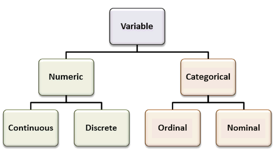
Recall the most common variable types. The types of the variables will define the analyses and visualizations that are possible.

Organize your data analysis project

To keep your files organized and easy to find, it’s a good idea to set up a clear naming system before you start collecting data for your thesis (or any other research-related data analysis).

A file naming convention is a consistent way to name files so it’s clear what’s inside and how each file connects to others. This helps you quickly understand and locate files, avoiding confusion or lost data later on.

1. Create a directory for the computatinal biology classes.

A key part of good data management is organizing your data effectively. This means planning how you’ll name files, arrange folders, and show relationships between them.
Researchers should set up folder structures that reflect how records were created and align with their workflows. Doing this improves clarity, makes it easier to save, find, and archive files, and supports collaboration across teams.

Establishing a clear file structure and naming system before collecting data ensures consistency and helps team members work more efficiently together.

We propose the following minimal structure inside a folder that identifies the :

project_nickname/    
├── data/    
│ ├── raw/    
│ └── processed/
│ └── metadata/    
├── scripts/    
├── output/    
└── docs/

project_nickname: root folder for the Rproject (for example: r_rep_data_analysis)
data/raw: original, unmodified data
data/processed: cleaned or transformed data ready for analysis
data/metadata: description of the contents in the data folder (learn more about metadata)
scripts: code for processing and analysis
output: figures, tables, and final results
docs: project documentation with supplementary files that are not data or analysis related

2. Create an RStudio project

RStudio Projects are a great functionality, easing the transition between dataset analyses, and allowing a fast navigation to your analysis/working directory. To create a new project:

File > New Project... > New Directory > New Project
Directory name: rep_data_analysis_r
Create a project as a subdirectory of: ~/
                           Browse... (folder that you created for the computational biology classes)
Create Project

Projects should be personalized by clicking on the menu in the right upper corner. The general options - R General - are the most important to customize, since they allow the definition of the RStudio “behavior” when the project is opened. The following suggestions are particularly useful:

Restore .RData at startup - No (for analyses with +1GB of data, you should choose "No")
Save .RData on exit - Ask
Always save history - Yes

3. Create a new R script file

In order to save your work, you must create a new R script file. Go to File > New File > R Script. A blank text file will appear above the console. Save it to your project folder with the name rep_data_analysis_mice.R

Why do we need scripts?

A script is a text file with a sequence of instructions that the computer runs to perform a task.

In R, you save the commands used in your analysis so you can run them again later. This makes your work reproducible, objective, and easy to update if the data change.

Although writing a script takes time at first, it allows you to work more efficiently in the long term. You can also share it with collaborators so they can review, improve, or extend your work. Many scientific journals now require authors to submit the analysis scripts with their manuscripts.

Load data and inspect it

Download the file mice_data.txt (mice weights according to diet) from here.
Create a folder named data inside your current working directory (where the RProject was created), and upload the mice_data.txt to the data folder.
Type the instructions inside grey boxes in pane number 2 of RStudio - the R Console. As you already know, the words after a # sign are comments not interpreted by R, so you do not need to copy them.
- In the R console, you must hit enter after each command to obtain the result.
- In the script file (R file), you must run the command by pressing the run button (on the top panel), or by selecting the code you want to run and pressing ctrl + enter.
Save all your relevant/final commands (R instructions) to your script file to be available for later use.

# Load the file and save it to object mice_data
mice_data <- read.table(file = "data/mice_data.txt", 
                        header = TRUE,
                        sep = "\t", 
                        dec = ".",
                        stringsAsFactors = TRUE)

# Briefly explore the dataset
View (mice_data)       # Open a tab in RStudio showing the whole table

head (mice_data, 10)   # Show the first 10 rows
tail (mice_data, 10)   # Show the last 10 rows
str(mice_data)         # Describe the class of each column in the dataset
summary (mice_data)    # Get the summary statistics for all columns

To facilitate further analysis, we will create 2 separate data frames: one for each type of diet.

# Filter the diet column by lean or fat and save results in a data frame
lean <- subset (mice_data, diet == "lean")
fat <- subset (mice_data, diet == "fat")

# Look at the new tables
head (lean)
head (fat)

Descriptive statistics and Plots using R

Now, we should look at the distributions of the variables. First we will use descriptive statistics that summarize the sample data. We will use measures of central tendency: Mean, Median, and Mode, and measures of dispersion (or variability): Standard Deviation, Variance, Maximum, and Minimum.

# Summary statistics per type of diet - min, max, median, average, standard deviation and variance 
summary(lean)      # quartiles, median, mean, max and min
sd (lean$weight)   # standard deviation of the weight
var(lean$weight)   # variance of the weight (var=sd^2)

summary(fat)
sd (fat$weight)   
var(fat$weight)

How is the variable “mouse weight” distributed in each diet? | Histograms

After summarizing the data, we should find appropriate plots to look at it. A first approach is to look at the frequency of the mouse weight values per diet using a histogram.

Recall Histograms

Histograms plot the distribution of a continuous variable (x-axis), in which the data is divided into a set of intervals (or bins), and the count (or frequency) of observations falling into each bin is plotted as the height of the bar.

# install.packages("ggplot2")       # package for plotting
# install.packages("RColorBrewer")  # color palettes
# install.packages("patchwork")     # combine plots

library(ggplot2)
library(RColorBrewer)
library(patchwork)

# Lean diet histogram
ggplot(lean, aes(x = weight)) +
  geom_histogram(
    binwidth = 5,
    color="white", 
    fill="skyblue1"
  ) +
  labs(
    x = "Mouse weight",
    title = "Lean Diet | Histogram of mouse weight",
    subtitle = "Binwidth = 5"
  ) +
  theme_minimal() -> lean_histogram    # save the plot

# Print the plot
lean_histogram

# Fat diet histogram
ggplot(fat, aes(x = weight)) +
  geom_histogram(
    binwidth = 1,
   color="white", 
    fill="seagreen3"
  ) +
  labs(
    x = "Mouse weight",
    title = "Fat Diet | Histogram of mouse weight",
    subtitle = "Binwidth = 1"
  ) +
  theme_minimal() -> fat_histogram    # save the plot

# Print the plot
fat_histogram

# Combine both histograms in the same plot using patchwork
  # Notice the different y axis scales
lean_histogram + fat_histogram

# Combine histograms with ggplot2 faceting
  # Axis scales can be formatted (the same or individual)
ggplot(mice_data, aes(x=weight, fill=diet)) +
  geom_histogram(binwidth=5, color="white") +
  facet_grid(~ diet)

How is the variable “mouse weight” distributed in each diet? | Boxplots

Since our data of interest is one categorical variable (type of diet), and one continuous variable (weight), a boxplot is one of the most informative.

Recall Boxplots

A boxplot represents the distribution of a continuous variable. The box in the middle represents the interquartile range (IQR), which is the range of values from the first quartile to the third quartile, and the line inside the box represents the median value (i.e. the second quartile). The lines extending from the box are called whiskers, and represent the range of the data outside the box, i.e. the maximum and the minimum, excluding any outliers, which are shown as points outside the whiskers (not present in this dataset). Outliers are defined as values that are more than 1.5 times the IQR below the first quartile or above the third quartile.

# Box and whiskers plot - BASIC
ggplot(mice_data, aes(x=diet, y=weight)) +
  geom_boxplot()

# Add color (from default ggplot palette)
ggplot(mice_data, aes(x=diet, y=weight)) +
  geom_boxplot(aes(fill=diet))

# Choose the colors, add X and Y axis names and the Title
    # Notice that the fill argument is not inside the aesthetics function
ggplot(mice_data, aes(x=diet, y=weight)) +
  geom_boxplot(fill=c("lightpink", "lightgreen")) +
  labs(x = "Diet",
       y = "Mouse weight (g)",
      title = "Boxplot of mouse weight"
    )

# Add points to the boxplot
ggplot(mice_data, aes(x = diet, y = weight)) +
  geom_boxplot(
    fill = c("lightpink", "lightgreen")
  ) +
  geom_jitter(
    width = 0.15,        # horizontal spread
    alpha = 0.7,         # transparency
    size = 2
  ) +
  labs(
    x = "Diet",
    y = "Mouse weight (g)",
    title = "Boxplot of mouse weight"
  )

How are the other variables distributed?

There are other variables in our data for each mouse that could influence the results, namely gender (categorical variable) and age (discrete variable). We should also look at these data.

Recall Barplots

A barplot represents the distribution of a categorical variable or the summary of a continuous variable across categories. Each bar corresponds to a category, and its height represents the value associated with that category, typically the count (frequency) or the proportion of observations.

When summarising a continuous variable, the height of the bar usually represents a summary statistic, such as the mean or the median, computed within each category.

The bars are separated by spaces to emphasise that the categories are discrete and do not have an intrinsic numerical continuity.

# Boxplot of diet and gender
ggplot(mice_data, aes(x=interaction(diet, gender), y=weight, 
                      fill=interaction(diet, gender))) +
  geom_boxplot() +
  geom_jitter(
    width = 0.15,        # horizontal spread
    alpha = 0.7,         # transparency
    size = 2             # point size
  ) +
  labs(
    x = "Diet and Gender interaction",
    y = "Mouse weight (g)",
    title = "Boxplot of mouse weights per diet type and gender"
  )

# Barplot of mice age
ggplot(mice_data, aes(x=age_months)) +
  geom_bar(fill="mediumpurple1",
           color="white") +
  labs(
    x = "Mice age (months)",
    y = "Count",
    title = "Barplot of mice age"
  ) +
  theme_light()  # simple and light background for the plot

What is the frequency of each variable?

When exploring the results of an experiment, we want to learn about the variables measured (age, gender, weight), and how many observations we have for each variable (number of females, number of males …), or combination of variables, for example, number of females in lean diet. This is easily done by using the function table. This function outputs a frequency table, i.e. the frequency (counts) of all combinations of the variables of interest.

# How many measurements do we have for each gender (a categorical variable)
table(mice_data$gender)

# How many measurements do we have for each diet (a categorical variable)
table(mice_data$diet)

# How many measurements do we have for each gender in each diet? 
  # (Count the number of observations in the combination between 
  # the two categorical variables).
table(mice_data$diet, mice_data$gender)

# We can also use this for numerical discrete variables, like age.
# How many measurements of each age (a discrete variable) do we have by gender? 
table(mice_data$age_months, mice_data$gender)

# And by diet type? 
table(mice_data$age_months, mice_data$diet)

# What if we want to know the results for each of the three variables:
  # age, diet and gender? Using ftable instead of table to format the
  # output in a more friendly way
ftable(mice_data$age_months, mice_data$diet, mice_data$gender)

Bivariate Analysis | Linear regression and Correlation coefficient

Is there a dependency between the age and the weight of the mice in our study?

To test if two variables are correlated we will start by:

Making a scatter plot of these two variables;
Followed by a calculation of the Pearson correlation coefficient;
Finally, fitting a linear model to the data to evaluate how the weight changes depending on the age of the mice.

# First step: scatter plot of age and weight 
# Note that the dependent variable is the weight, so it should be in the y axis,
  # and the independent variable (age) should be in the x axis.
ggplot(mice_data, aes(x=age_months, y=weight)) +
  geom_point(shape=19, size=2)

# Second step: Calculate the Pearson coefficient of correlation (r)
my.correlation <- cor(mice_data$weight, 
                      mice_data$age_months, 
                      method = "pearson")
my.correlation

# Third step: fit a linear model (using the function lm) to check the coefficients overall
my.lm <- lm (weight ~ age_months, data=mice_data) 
my.lm

# Fit a line with confidence interval
ggplot(mice_data, aes(x = age_months, y = weight)) +
  geom_point(shape = 19, size = 2.5, alpha = 0.7) +
  geom_smooth(method = "lm", se = TRUE, formula = y ~ x) +
  labs(
    y = "Weight (g) [Dependent variable]",
    x = "Age (months) [Independent variable]"
  )

# Fit one line per diet type
  # Just add a color grouping and ggplot fits one line per group
ggplot(mice_data, aes(x = age_months, y = weight, color = diet)) +
  geom_point(shape = 19, size = 2.5, alpha = 0.7) +
  geom_smooth(method = "lm", se = FALSE, formula = y ~ x) +
  labs(
    y = "Weight (g) [Dependent variable]",
    x = "Age (months) [Independent variable]",
    color = "Diet"
  )

Hypothesis testing and Statistical significance using R

Going back to our original question: Does the type of diet influence the body weight of mice?
Can we answer this question just by looking at the plot? Are these observations compatible with a scenario where the type of diet does not influence body weight?

Remember the basic statistical methods:

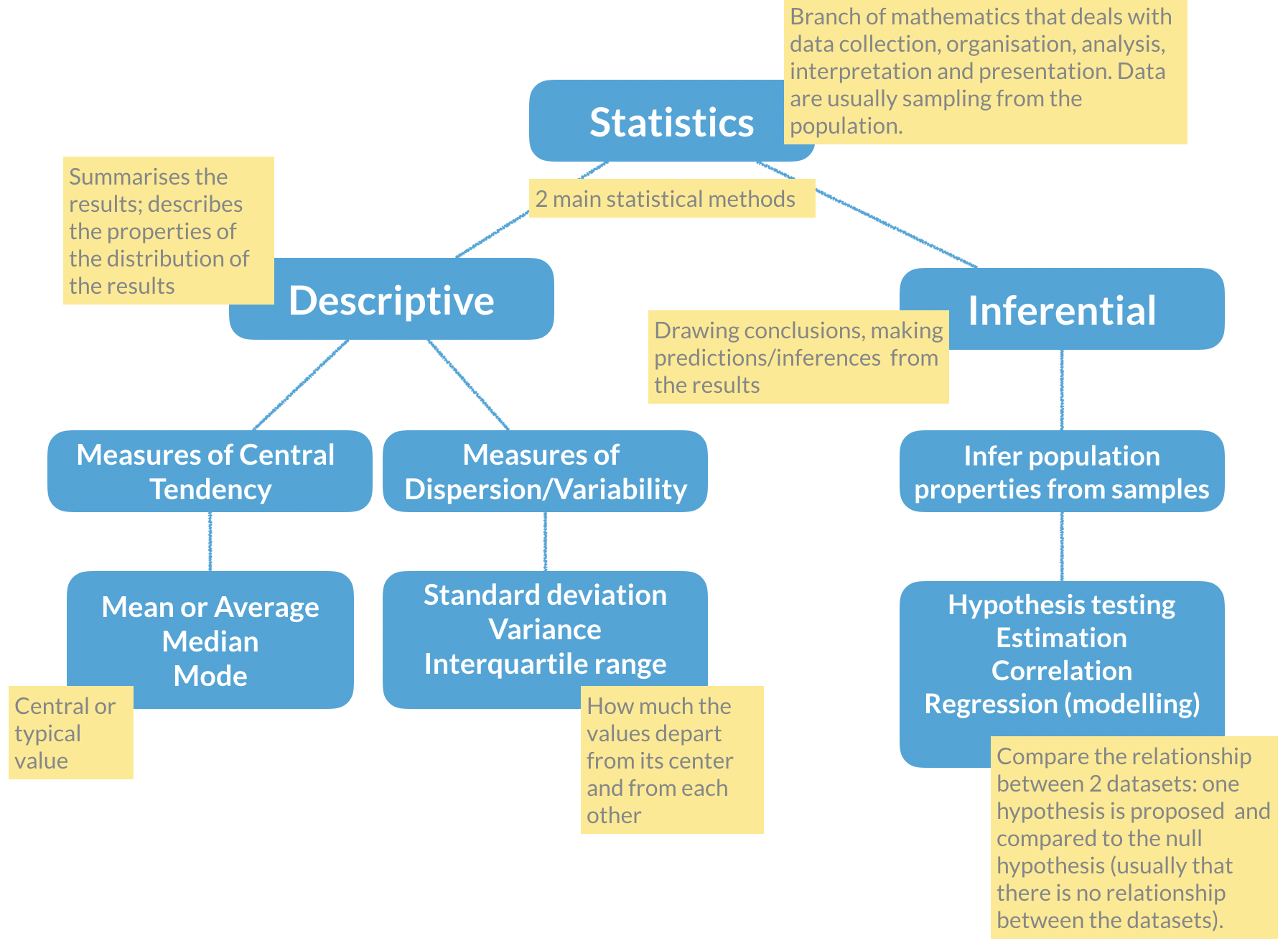
Here enters hypothesis testing. In hypothesis testing, the investigator formulates a null hypothesis (H0) that usually states that there is no difference between the two groups, i.e. the observed weight differences between the two groups of mice occurred only due to sampling fluctuations (like when you repeat an experiment drawing samples from the same population). In other words, H0 corresponds to an absence of effect.
The alternative hypothesis (H1), just states that the effect is present between the two groups, i.e. that the samples were taken from different populations.

Hypothesis testing proceeds with using a statistical test to try and reject H0. For this experiment, we will use a T-test that compares the difference between the means of the two diet groups, yielding a p-value that we will use to decide if we reject the null hypothesis, at a 5% significance level (p-value < 0.05). Meaning that, if we repeat this experiment 100 times in different mice, in 5 of those experiments we will reject the null hypothesis, even thought the null hypothesis is true.

# Apply a T-test to the lean and fat diet weights 

### Explanation of the arguments used ###
  # alternative="two.sided": two-sided because we want to test any difference 
  # between the means, and not only weight gain or weight loss 
  # (in which case it would be a one-sided test)

  # paired=FALSE: because we measured the weight in 2 different groups of mice
  # (never the same individual). If we measure a variable 2 times in the same
  # individual the data would be paired.

  # var.equal=TRUE: T-tests apply to equal variance data, so we assume it is
  # TRUE and ask R to estimate the variance (if we chose FALSE, then R uses
  # another similar method called Welch (or Satterthwaite) approximation) 

ttest <- t.test(lean$weight, fat$weight,
                alternative="two.sided", 
                paired = FALSE, 
                var.equal = TRUE)

# Print the results
ttest

Now that we have calculated the T-test, shall we accept or reject the null hypothesis? What are the outputs in R from the t-test?

# Find the names of the output from the function t.test
names(ttest)

# Extract just the p-value
ttest$p.value

Final discussion

Take some time to discuss the results with your classmates, and decide if H0 should be rejected or not, and how confident you are that your decision is reasonable. Can you propose solutions to improve your confidence on the results? Is the experimental design appropriate for the research question being asked? Is this experiment well controlled and balanced?

Advanced mini-project

The Topic 2 | Advanced R mini-project is a hands-on tutorial that walks you through the complete workflow of reproducible data analysis in R, from organizing your project, and cleaning/tidying your dataset, to applying machine learning to your data.

Enjoy!

R Intro

Learning R: Tutorials and Mini-projects

1. Using RStudio

2. Load the swirl package & Follow the guided course

Hands-on Tutorial

Setting up Your Workspace

RStudio as Your R Environment

Creating an RStudio Project

Your Working Directory

Saving and Quitting

Packages: Extending What R Can Do

What Is a Package?

Installing and Loading Packages

Getting Help

Operators

Arithmetic Operators

Assignment Operators

Comparison Operators

Logical Operators

The Pipe Operator

R’s Five Core Data Structures

Vectors

Matrices

Data Frames

Lists

Factors

Converting Between Data Structures

Control Flow: Loops and Conditionals

for Loops

while Loops

if / else Conditionals

ifelse() - Vectorised Conditionals

The apply() Family of Functions

apply() - Over Rows or Columns of a Matrix or Data Frame

lapply() - Over a List, Always Returns a List

sapply() is like lapply(), but Simplifies the Result

Comparison: Loop vs Apply

Writing Your Own Functions

Function Syntax

A Worked Example

Default Argument Values

Loading Data and Saving Results

Writing Data to Files

Reading Data from Files

Modern Alternatives

A Tour of Useful Built-in Functions

Exploring a Dataset

Descriptive Statistics

Counting, Grouping and Summarising

Filtering and Selecting

Sorting and Ordering

Logical Tests on Vectors

Combining Data Frames

Mathematical Functions

Working with Categorical Data: cut()

Where to Go From Here

Descriptive statistics in R

Start by discussing the experimental design

Organize your data analysis project

Load data and inspect it

Descriptive statistics and Plots using R

How is the variable “mouse weight” distributed in each diet? | Histograms

How is the variable “mouse weight” distributed in each diet? | Boxplots

How are the other variables distributed?

What is the frequency of each variable?

Bivariate Analysis | Linear regression and Correlation coefficient

Hypothesis testing and Statistical significance using R

Now that we have calculated the T-test, shall we accept or reject the null hypothesis? What are the outputs in R from the t-test?

Final discussion

Advanced mini-project

**2. Load the swirl package & Follow the guided course**

`for` Loops

`while` Loops

`if` / `else` Conditionals

`ifelse()` - Vectorised Conditionals

The `apply()` Family of Functions

`apply()` - Over Rows or Columns of a Matrix or Data Frame

`lapply()` - Over a List, Always Returns a List

`sapply()` is like `lapply()`, but Simplifies the Result

Working with Categorical Data: `cut()`