# Create the folder structure for the project
dir.create("data/raw", recursive = TRUE)
dir.create("data/processed", recursive = TRUE)
dir.create("scripts", recursive = TRUE)
dir.create("output/figures", recursive = TRUE)
dir.create("output/tables", recursive = TRUE)
dir.create("docs", recursive = TRUE)Topic 2 | Advanced R
Reproducible Data Analysis: From Messy Data to Machine Learning
Overview
Mini-Project Details
Estimated time: 3–4 hours
Synopsis: This hands-on mini-project walks you through the complete workflow of reproducible data analysis in R, from organizing your project to applying machine learning techniques.
In this mini-project, you will:
- Set up a proper folder structure for reproducible research
- Load and inspect a messy dataset
- Clean and tidy the data following best practices
- Perform exploratory data analysis with descriptive statistics
- Create publication-quality visualizations with ggplot2
- Apply dimensionality reduction with PCA
- Build a simple machine learning model using tidymodels
We will work with a messy version of the Palmer Penguins dataset, a popular alternative to the iris dataset for learning data science. The data contains measurements of penguins from three species observed on three islands in the Palmer Archipelago, Antarctica.
1 Part 1: Project Setup and Organization
A well-organized project structure is the foundation of reproducible research. Before writing any code, we establish a clear directory hierarchy.
1.1 Create the project folder structure
Open RStudio and create a new project:
File > New Project... > New Directory > New Project
Directory name: penguins_analysis
Create project as subdirectory of: ~/
Create Project
Now create the required subdirectories. Run this in the R console:
Your project should now have this structure:
penguins_analysis/
├── data/
│   ├── raw/           # Original, unmodified data
│   └── processed/     # Cleaned data ready for analysis
├── scripts/           # R scripts for data processing
├── output/
│   ├── figures/       # Plots and visualizations
│   └── tables/        # Summary tables
├── docs/              # Documentation and notes
└── penguins_analysis.Rproj
Why this structure?
- raw/: Never modify original data. Keep it read-only as a reference.
- processed/: Store cleaned versions with clear names.
- scripts/: Separate data cleaning from analysis for clarity.
- output/: Makes it easy to regenerate all results from code.
1.2 Download the messy dataset
Download the messy_penguins.csv file from the course materials and place it in the data/raw/ folder.
The file is available at: messy_penguins.csv
2 Part 2: Loading and Inspecting Messy Data
2.1 Load required packages
We use the tidyverse ecosystem for modern, readable R code:
# Core tidyverse packages
library(tidyverse)   # includes ggplot2, dplyr, tidyr, readr, etc.

# Additional packages for this project
library(janitor)     # data cleaning utilities
library(skimr)       # summary statistics
library(corrplot)    # correlation visualization
library(GGally)      # pairs plots
library(tidymodels)
If any package is not installed, run:
install.packages(c("tidyverse", "janitor", "skimr", "corrplot",
                   "GGally", "tidymodels", "ranger"))
2.2 Read the messy data
Always use explicit arguments when reading data to ensure reproducibility:
# Read the messy data from the raw folder
penguins_raw <- read_csv(
  "data/raw/messy_penguins.csv",
  col_types = cols(.default = col_character()),  # read all as character first
  na = c("", "NA", "na", "N/A", "n/a", "missing") # define missing values
)

# First look at the data
penguins_raw
# A tibble: 120 × 9
ID Species island bill_length_mm bill_depth_mm `flipper_length (mm)`
<chr> <chr> <chr> <chr> <chr> <chr>
1 1 Adelie Torgersen 39.1 18.7 181
2 2 adelie Torgersen 39.5 17.4 186
3 3 Adelie Torgersen 40.3 18 195
4 4 Adelie Torgersen <NA> <NA> <NA>
5 5 ADELIE Torgersen 36.7 19.3 193
6 6 Adelie Torgersen 39.3 20.6 190
7 7 Adelie Torgersen 38.9 17.8 181
8 8 Adelie torgersen 39.2 19.6 195
9 9 Adelie Torgersen 34.1 18.1 193
10 10 Adelie Torgersen 42 20.2 190
# ℹ 110 more rows
# ℹ 3 more variables: `body mass (g)` <chr>, Sex <chr>, year <chr>2.3 Inspect the data structure
Before cleaning, we need to understand what problems exist:
# Check dimensions
dim(penguins_raw)
[1] 120 9# View column names (notice the inconsistent naming)
names(penguins_raw)[1] "ID" "Species" "island"
[4] "bill_length_mm" "bill_depth_mm" "flipper_length (mm)"
[7] "body mass (g)" "Sex" "year" # Check the structure
str(penguins_raw)spc_tbl_ [120 × 9] (S3: spec_tbl_df/tbl_df/tbl/data.frame)
$ ID : chr [1:120] "1" "2" "3" "4" ...
$ Species : chr [1:120] "Adelie" "adelie" "Adelie" "Adelie" ...
$ island : chr [1:120] "Torgersen" "Torgersen" "Torgersen" "Torgersen" ...
$ bill_length_mm : chr [1:120] "39.1" "39.5" "40.3" NA ...
$ bill_depth_mm : chr [1:120] "18.7" "17.4" "18" NA ...
$ flipper_length (mm): chr [1:120] "181" "186" "195" NA ...
$ body mass (g) : chr [1:120] "3750" "3800" "3250" NA ...
$ Sex : chr [1:120] "male" "FEMALE" "Female" NA ...
$ year : chr [1:120] "2007" "2007" "2007" "2007" ...
- attr(*, "spec")=
.. cols(
.. .default = col_character(),
.. ID = col_character(),
.. Species = col_character(),
.. island = col_character(),
.. bill_length_mm = col_character(),
.. bill_depth_mm = col_character(),
.. `flipper_length (mm)` = col_character(),
.. `body mass (g)` = col_character(),
.. Sex = col_character(),
.. year = col_character()
.. )
- attr(*, "problems")=<externalptr> # Quick glimpse
glimpse(penguins_raw)Rows: 120
Columns: 9
$ ID <chr> "1", "2", "3", "4", "5", "6", "7", "8", "9", "10…
$ Species <chr> "Adelie", "adelie", "Adelie", "Adelie", "ADELIE"…
$ island <chr> "Torgersen", "Torgersen", "Torgersen", "Torgerse…
$ bill_length_mm <chr> "39.1", "39.5", "40.3", NA, "36.7", "39.3", "38.…
$ bill_depth_mm <chr> "18.7", "17.4", "18", NA, "19.3", "20.6", "17.8"…
$ `flipper_length (mm)` <chr> "181", "186", "195", NA, "193", "190", "181", "1…
$ `body mass (g)` <chr> "3750", "3800", "3250", NA, "3450", "3650", "362…
$ Sex <chr> "male", "FEMALE", "Female", NA, "female", "Male"…
$ year <chr> "2007", "2007", "2007", "2007", "2007", "2007", …2.4 Identify data quality issues
Let’s systematically check for problems:
# Check unique values in categorical columns
penguins_raw |>
  count(Species, sort = TRUE)
# A tibble: 9 × 2
Species n
<chr> <int>
1 Adelie 41
2 Gentoo 32
3 Chinstrap 24
4 adelie 5
5 ADELIE 4
6 GENTOO 4
7 gentoo 4
8 CHINSTRAP 3
9 chinstrap 3penguins_raw |>
count(island, sort = TRUE)# A tibble: 6 × 2
island n
<chr> <int>
1 Biscoe 46
2 Dream 37
3 Torgersen 28
4 biscoe 4
5 dream 3
6 torgersen 2penguins_raw |>
count(Sex, sort = TRUE)# A tibble: 6 × 2
Sex n
<chr> <int>
1 Male 29
2 male 28
3 female 21
4 Female 19
5 FEMALE 18
6 <NA> 5# Check for missing values
penguins_raw |>
summarise(across(everything(), ~ sum(is.na(.))))# A tibble: 1 × 9
ID Species island bill_length_mm bill_depth_mm `flipper_length (mm)`
<int> <int> <int> <int> <int> <int>
1 0 0 0 2 2 2
# ℹ 3 more variables: `body mass (g)` <int>, Sex <int>, year <int>
Data Quality Issues Identified
- Column names: Inconsistent formatting (spaces, parentheses, mixed case)
- Species: Mixed case (“Adelie”, “adelie”, “ADELIE”)
- Island: Mixed case (“Torgersen”, “torgersen”, “Biscoe”, “biscoe”)
- Sex: Multiple representations (“male”, “Male”, “MALE”, “female”, “Female”, “FEMALE”)
- Missing values: Multiple representations already converted to NA
- Numeric columns: Currently stored as character
- Incomplete rows: Row 39 is missing the last columns
3 Part 3: Data Cleaning and Tidying
Now we create a reproducible cleaning script. This script should be saved separately in scripts/clean_penguins.R for reuse.
3.1 Step-by-step cleaning
penguins_clean <- penguins_raw |>
  # Step 1: Clean column names (snake_case, lowercase)
  janitor::clean_names() |>

  # Step 2: Rename columns with units in the name
  rename(
    flipper_length_mm = flipper_length_mm,
    body_mass_g = body_mass_g
  ) |>

  # Step 3: Standardize categorical variables
  mutate(
    species = str_to_title(species),    # Capitalize first letter
    island = str_to_title(island),
    sex = str_to_lower(sex),
    sex = case_when(
      sex %in% c("male", "m") ~ "male",
      sex %in% c("female", "f") ~ "female",
      TRUE ~ NA_character_
    )
  ) |>

  # Step 4: Convert numeric columns
  mutate(
    bill_length_mm = as.numeric(bill_length_mm),
    bill_depth_mm = as.numeric(bill_depth_mm),
    flipper_length_mm = as.numeric(flipper_length_mm),
    body_mass_g = as.numeric(body_mass_g),
    year = as.integer(year)
  ) |>

  # Step 5: Convert to factors where appropriate
  mutate(
    species = factor(species),
    island = factor(island),
    sex = factor(sex)
  ) |>

  # Step 6: Remove the ID column (not needed for analysis)
  select(-id) |>

  # Step 7: Remove rows with all measurements missing
  filter(!if_all(c(bill_length_mm, bill_depth_mm,
                   flipper_length_mm, body_mass_g), is.na))

# Check the result
glimpse(penguins_clean)
Rows: 118
Columns: 8
$ species <fct> Adelie, Adelie, Adelie, Adelie, Adelie, Adelie, Adel…
$ island <fct> Torgersen, Torgersen, Torgersen, Torgersen, Torgerse…
$ bill_length_mm <dbl> 39.1, 39.5, 40.3, 36.7, 39.3, 38.9, 39.2, 34.1, 42.0…
$ bill_depth_mm <dbl> 18.7, 17.4, 18.0, 19.3, 20.6, 17.8, 19.6, 18.1, 20.2…
$ flipper_length_mm <dbl> 181, 186, 195, 193, 190, 181, 195, 193, 190, 186, 18…
$ body_mass_g <dbl> 3750, 3800, 3250, 3450, 3650, 3625, 4675, 3475, 4250…
$ sex <fct> male, female, female, female, male, female, male, NA…
$ year <int> 2007, 2007, 2007, 2007, 2007, 2007, 2007, 2007, 2007…3.2 Validate the cleaned data
# Check factor levels
levels(penguins_clean$species)
[1] "Adelie" "Chinstrap" "Gentoo" levels(penguins_clean$island)[1] "Biscoe" "Dream" "Torgersen"levels(penguins_clean$sex)[1] "female" "male" # Summary of numeric variables
penguins_clean |>
select(where(is.numeric)) |>
summary() bill_length_mm bill_depth_mm flipper_length_mm body_mass_g
Min. :34.10 Min. :13.20 Min. :172.0 Min. :2700
1st Qu.:39.50 1st Qu.:15.32 1st Qu.:187.0 1st Qu.:3631
Median :45.70 Median :17.80 Median :195.0 Median :3900
Mean :44.36 Mean :17.28 Mean :198.4 Mean :4210
3rd Qu.:48.70 3rd Qu.:18.70 3rd Qu.:212.8 3rd Qu.:4769
Max. :58.00 Max. :21.50 Max. :230.0 Max. :6300
year
Min. :2007
1st Qu.:2007
Median :2007
Mean :2007
3rd Qu.:2007
Max. :2008 # Use skimr for a comprehensive summary
skim(penguins_clean)| Name | penguins_clean |
| Number of rows | 118 |
| Number of columns | 8 |
| _______________________ | |
| Column type frequency: | |
| factor | 3 |
| numeric | 5 |
| ________________________ | |
| Group variables | None |
Variable type: factor
| skim_variable | n_missing | complete_rate | ordered | n_unique | top_counts |
|---|---|---|---|---|---|
| species | 0 | 1.00 | FALSE | 3 | Ade: 48, Gen: 40, Chi: 30 |
| island | 0 | 1.00 | FALSE | 3 | Bis: 50, Dre: 40, Tor: 28 |
| sex | 3 | 0.97 | FALSE | 2 | fem: 58, mal: 57 |
Variable type: numeric
| skim_variable | n_missing | complete_rate | mean | sd | p0 | p25 | p50 | p75 | p100 | hist |
|---|---|---|---|---|---|---|---|---|---|---|
| bill_length_mm | 0 | 1 | 44.36 | 5.18 | 34.1 | 39.50 | 45.7 | 48.70 | 58.0 | ▅▆▇▇▁ |
| bill_depth_mm | 0 | 1 | 17.28 | 2.09 | 13.2 | 15.33 | 17.8 | 18.70 | 21.5 | ▅▃▆▇▂ |
| flipper_length_mm | 0 | 1 | 198.45 | 14.40 | 172.0 | 187.00 | 195.0 | 212.75 | 230.0 | ▃▇▃▅▂ |
| body_mass_g | 0 | 1 | 4209.53 | 813.92 | 2700.0 | 3631.25 | 3900.0 | 4768.75 | 6300.0 | ▂▇▃▂▂ |
| year | 0 | 1 | 2007.25 | 0.43 | 2007.0 | 2007.00 | 2007.0 | 2007.00 | 2008.0 | ▇▁▁▁▂ |
3.3 Save the cleaned data
# Save to processed folder
write_csv(penguins_clean, "data/processed/penguins_clean.csv")

# Confirmation message
cat("Cleaned data saved to: data/processed/penguins_clean.csv\n")
Cleaned data saved to: data/processed/penguins_clean.csvcat("Original rows:", nrow(penguins_raw), "\n")Original rows: 120 cat("Cleaned rows:", nrow(penguins_clean), "\n")Cleaned rows: 118 4 Part 4: Exploratory Data Analysis | Descriptive Statistics
Now we explore the cleaned data to understand its characteristics before any modeling.
4.1 Load the cleaned data
In a real workflow, you would start here if the cleaning was done previously:
4.2 Sample size by group
penguins <- read_csv(
  "data/processed/penguins_clean.csv",
  col_types = cols(
    species = col_character(),
    island = col_character(),
    sex = col_character(),
    bill_length_mm = col_double(),
    bill_depth_mm = col_double(),
    flipper_length_mm = col_double(),
    body_mass_g = col_double(),
    year = col_integer()
  )
) |>
  mutate(
    species = factor(species),
    island = factor(island),
    sex = factor(sex)
  )
4.3 Summary statistics by species
# Calculate descriptive statistics for numeric variables by species
penguins |>
  group_by(species) |>
  summarise(
    n = n(),
    mean_bill_length = mean(bill_length_mm, na.rm = TRUE),
    sd_bill_length = sd(bill_length_mm, na.rm = TRUE),
    mean_bill_depth = mean(bill_depth_mm, na.rm = TRUE),
    sd_bill_depth = sd(bill_depth_mm, na.rm = TRUE),
    mean_flipper_length = mean(flipper_length_mm, na.rm = TRUE),
    sd_flipper_length = sd(flipper_length_mm, na.rm = TRUE),
    mean_body_mass = mean(body_mass_g, na.rm = TRUE),
    sd_body_mass = sd(body_mass_g, na.rm = TRUE)
  ) |>
  mutate(across(where(is.numeric), ~ round(., 2)))
# A tibble: 3 × 10
species n mean_bill_length sd_bill_length mean_bill_depth sd_bill_depth
<fct> <dbl> <dbl> <dbl> <dbl> <dbl>
1 Adelie 48 39.0 2.32 18.7 1.18
2 Chinstrap 30 49.1 2.89 18.4 0.96
3 Gentoo 40 47.2 2.48 14.8 0.88
# ℹ 4 more variables: mean_flipper_length <dbl>, sd_flipper_length <dbl>,
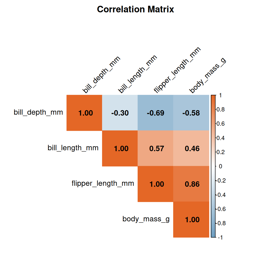
# mean_body_mass <dbl>, sd_body_mass <dbl>4.4 Correlation analysis
# Calculate correlation matrix for numeric variables
cor_matrix <- penguins |>
  select(where(is.numeric), -year) |>
  drop_na() |>
  cor()

# Display the correlation matrix
round(cor_matrix, 2)
bill_length_mm bill_depth_mm flipper_length_mm body_mass_g
bill_length_mm 1.00 -0.30 0.57 0.46
bill_depth_mm -0.30 1.00 -0.69 -0.58
flipper_length_mm 0.57 -0.69 1.00 0.86
body_mass_g 0.46 -0.58 0.86 1.005 Part 5: Data Visualization with ggplot2
Visualization is essential for understanding patterns in data. We follow the grammar of graphics principles.
5.1 Distribution of measurements
# Histograms of all numeric variables
penguins |>
  select(species, bill_length_mm, bill_depth_mm,
         flipper_length_mm, body_mass_g) |>
  pivot_longer(
    cols = -species,
    names_to = "measurement",
    values_to = "value"
  ) |>
  ggplot(aes(x = value, fill = species)) +
  geom_histogram(bins = 20, alpha = 0.7, position = "identity") +
  facet_wrap(~ measurement, scales = "free") +
  scale_fill_brewer(palette = "Set2") +
  labs(
    title = "Distribution of Penguin Measurements",
    x = "Value",
    y = "Count",
    fill = "Species"
  ) +
  theme_minimal() +
  theme(legend.position = "bottom")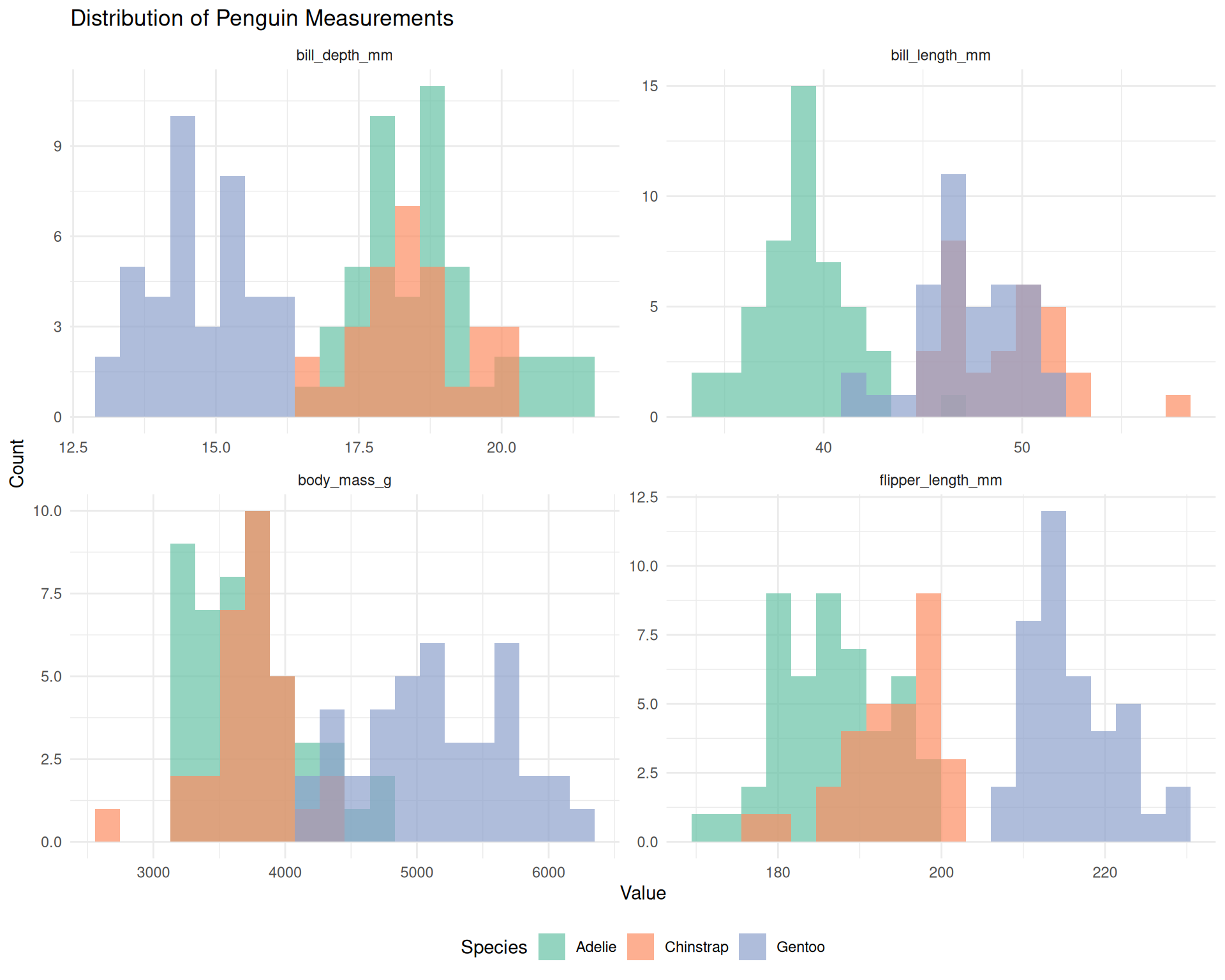
5.2 Boxplots comparing species
ggplot(penguins, aes(x = species, y = body_mass_g, fill = species)) +
  geom_boxplot(alpha = 0.7, outlier.shape = NA) +
  geom_jitter(width = 0.2, alpha = 0.4, size = 1.5) +
  scale_fill_brewer(palette = "Set2") +
  labs(
    title = "Body Mass Distribution by Species",
    x = "Species",
    y = "Body Mass (g)"
  ) +
  theme_minimal() +
  theme(legend.position = "none")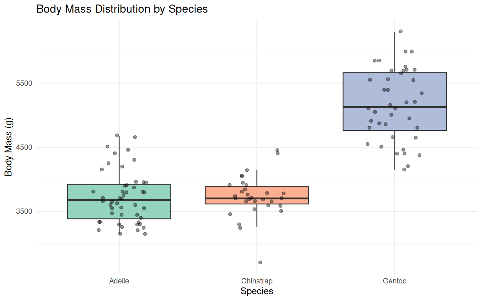
5.3 Scatter plot with regression lines
ggplot(penguins, aes(x = bill_length_mm, y = bill_depth_mm, color = species)) +
  geom_point(alpha = 0.7, size = 2) +
  geom_smooth(method = "lm", se = TRUE, alpha = 0.2) +
  scale_color_brewer(palette = "Set2") +
  labs(
    title = "Bill Length vs Bill Depth",
    subtitle = "Within-species positive correlations",
    x = "Bill Length (mm)",
    y = "Bill Depth (mm)",
    color = "Species"
  ) +
  theme_minimal() +
  theme(legend.position = "bottom")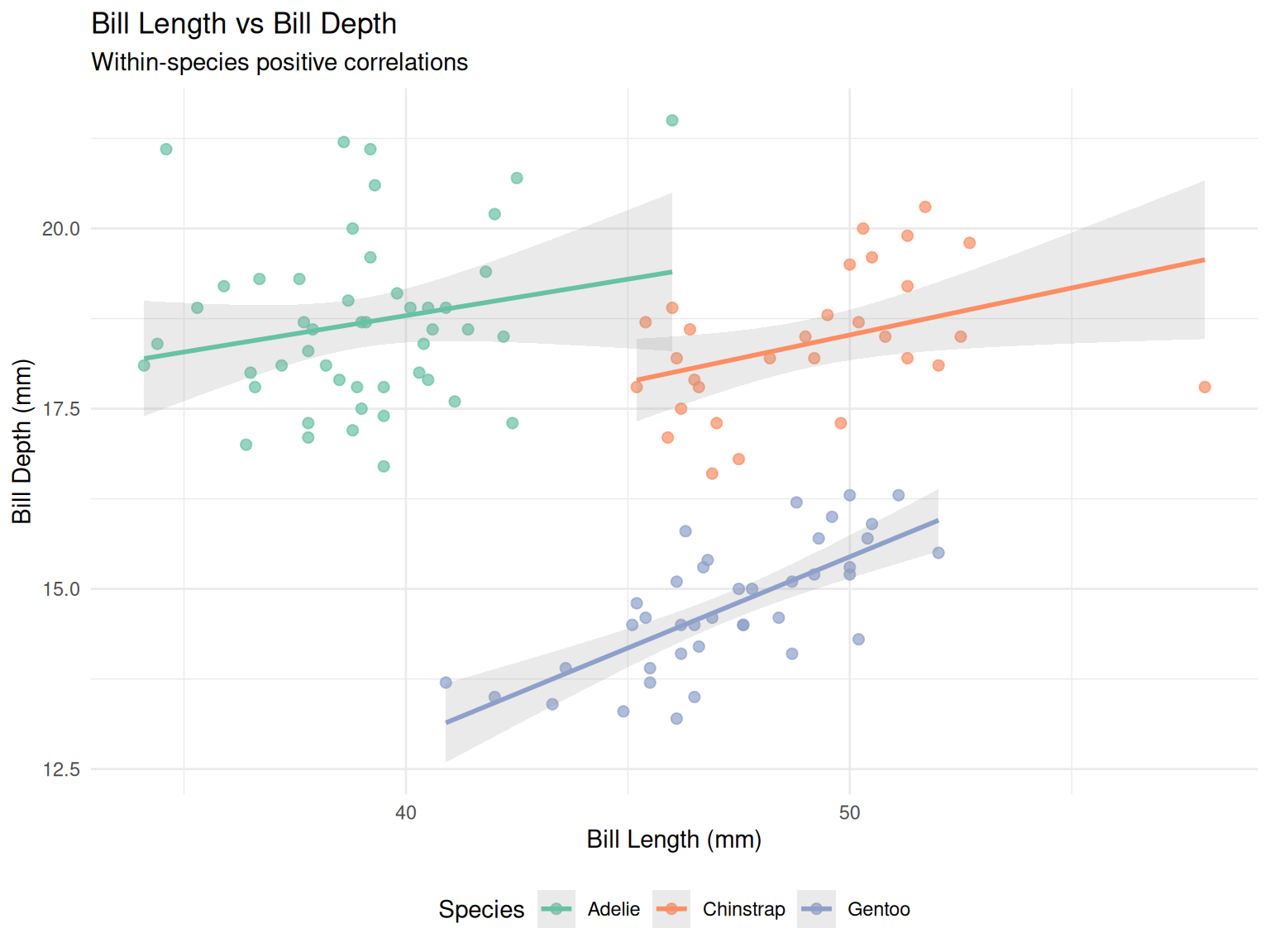
Simpson’s paradox
This dataset is well know for displaying an instance of Simpson’s paradox for the relationship between bill dimensions, where it presents an overall negative correlation (when no stratification by species is performed); but this trend is reversed when looking at individual species (which present whithin-species positive correlation).
5.4 Pairs plot for multivariate exploration
penguins |>
  select(species, bill_length_mm, bill_depth_mm,
         flipper_length_mm, body_mass_g) |>
  drop_na() |>
  ggpairs(
    columns = 2:5,
    mapping = aes(color = species, alpha = 0.5),
    upper = list(continuous = wrap("cor", size = 3)),
    lower = list(continuous = wrap("points", size = 1)),
    diag = list(continuous = wrap("densityDiag", alpha = 0.5))
  ) +
  scale_color_brewer(palette = "Set2") +
  scale_fill_brewer(palette = "Set2") +
  theme_minimal()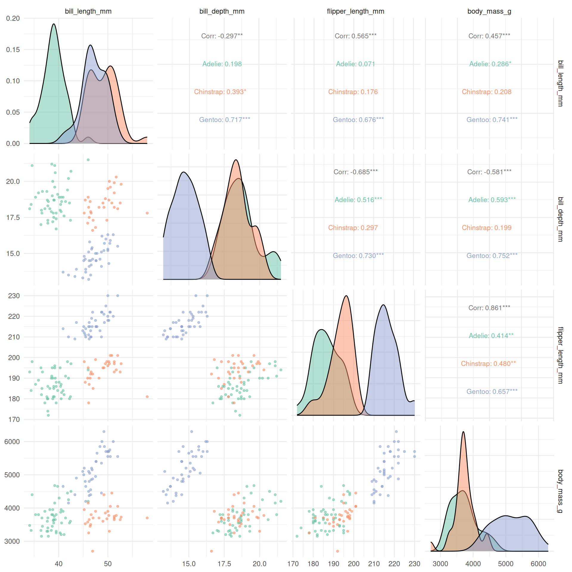
5.5 Correlation heatmap
corrplot(
  cor_matrix,
  method = "color",
  type = "upper",
  order = "hclust",
  addCoef.col = "black",
  tl.col = "black",
  tl.srt = 45,
  col = colorRampPalette(c("#6D9EC1", "white", "#E46726"))(200),
  title = "Correlation Matrix",
  mar = c(0, 0, 2, 0)
)
6 Part 6: Principal Component Analysis (PCA)
PCA reduces dimensionality while preserving variance, useful for visualization and understanding variable relationships.
6.1 Prepare data for PCA
# PCA requires complete cases and only numeric variables
penguins_pca_data <- penguins |>
  select(species, bill_length_mm, bill_depth_mm,
         flipper_length_mm, body_mass_g) |>
  drop_na()

# Extract numeric columns and scale them
penguins_scaled <- penguins_pca_data |>
  select(-species) |>
  scale()

# Store species for later plotting
species_labels <- penguins_pca_data$species
6.2 Perform PCA
# Run PCA
pca_result <- prcomp(penguins_scaled, center = FALSE, scale. = FALSE)

# Summary of PCA
summary(pca_result)
Importance of components:
PC1 PC2 PC3 PC4
Standard deviation 1.6623 0.8473 0.6374 0.33541
Proportion of Variance 0.6908 0.1795 0.1016 0.02813
Cumulative Proportion 0.6908 0.8703 0.9719 1.000006.3 Variance explained
# Calculate variance explained
var_explained <- tibble(
  PC = paste0("PC", 1:4),
  variance = pca_result$sdev^2,
  prop_variance = variance / sum(variance),
  cum_variance = cumsum(prop_variance)
)

var_explained
# A tibble: 4 × 4
PC variance prop_variance cum_variance
<chr> <dbl> <dbl> <dbl>
1 PC1 2.76 0.691 0.691
2 PC2 0.718 0.179 0.870
3 PC3 0.406 0.102 0.972
4 PC4 0.113 0.0281 1 # Scree plot
ggplot(var_explained, aes(x = PC, y = prop_variance)) +
geom_col(fill = "steelblue", alpha = 0.7) +
geom_line(aes(group = 1), color = "darkred", linewidth = 1) +
geom_point(color = "darkred", size = 3) +
geom_text(aes(label = scales::percent(prop_variance, accuracy = 0.1)),
vjust = -0.5) +
scale_y_continuous(labels = scales::percent) +
labs(
title = "Variance Explained by Principal Components",
x = "Principal Component",
y = "Proportion of Variance"
) +
theme_minimal()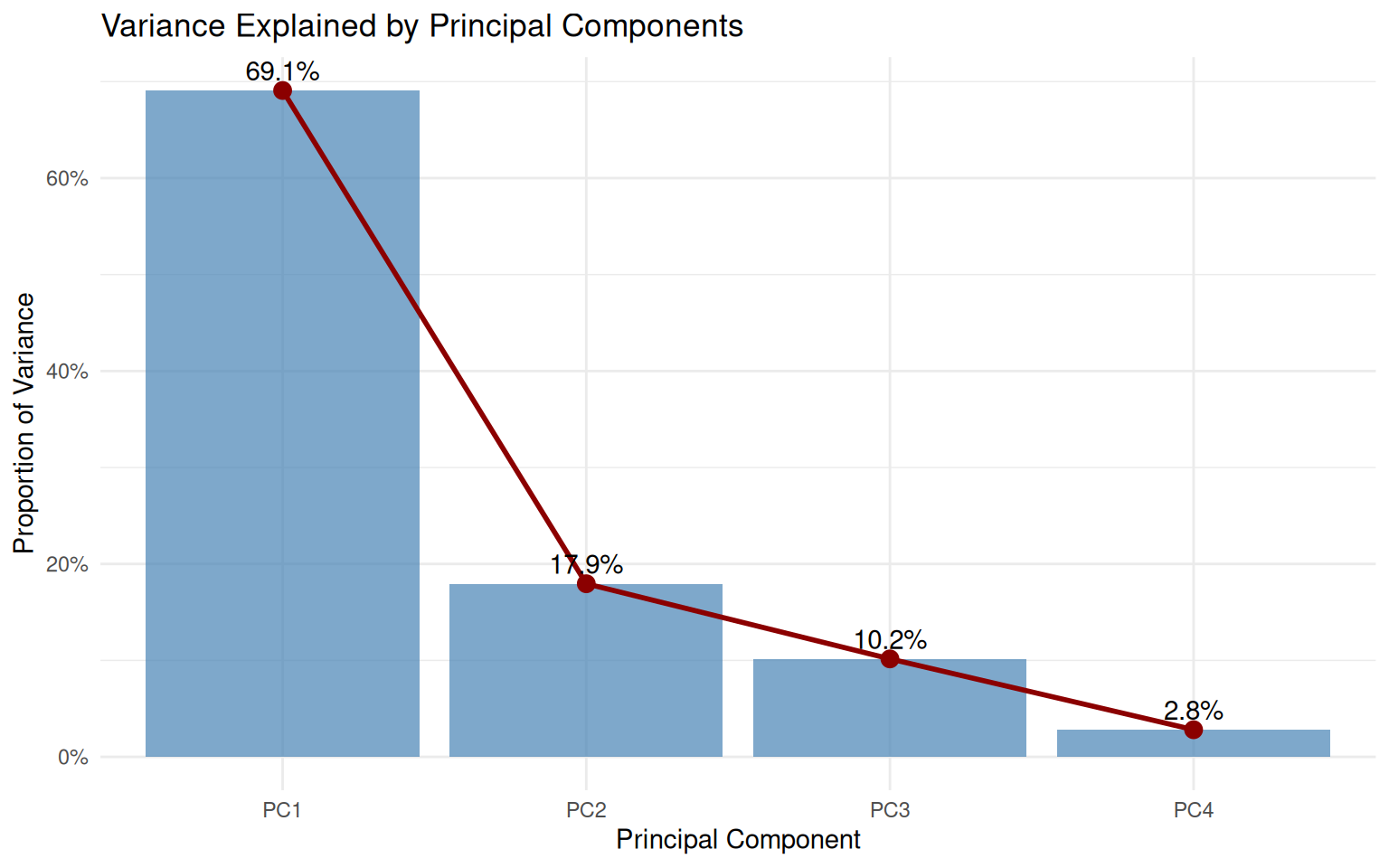
6.4 PCA biplot
# Create data frame with PC scores
pca_scores <- as_tibble(pca_result$x) |>
  mutate(species = species_labels)

# Loadings for arrows
loadings <- as_tibble(pca_result$rotation, rownames = "variable") |>
  mutate(
    PC1 = PC1 * 3,  # scale for visibility
    PC2 = PC2 * 3
  )

# Biplot
ggplot() +
  # Points colored by species
  geom_point(
    data = pca_scores,
    aes(x = PC1, y = PC2, color = species),
    alpha = 0.7, size = 2
  ) +
  # Loadings as arrows
  geom_segment(
    data = loadings,
    aes(x = 0, y = 0, xend = PC1, yend = PC2),
    arrow = arrow(length = unit(0.2, "cm")),
    color = "gray30", linewidth = 0.8
  ) +
  # Labels for loadings
  geom_text(
    data = loadings,
    aes(x = PC1 * 1.1, y = PC2 * 1.1, label = variable),
    color = "gray20", size = 3.5
  ) +
  scale_color_brewer(palette = "Set2") +
  labs(
    title = "PCA Biplot of Penguin Measurements",
    subtitle = paste0("PC1 + PC2 explain ",
                      scales::percent(sum(var_explained$prop_variance[1:2]),
                                     accuracy = 0.1),
                      " of variance"),
    x = paste0("PC1 (", scales::percent(var_explained$prop_variance[1],
                                        accuracy = 0.1), ")"),
    y = paste0("PC2 (", scales::percent(var_explained$prop_variance[2],
                                        accuracy = 0.1), ")"),
    color = "Species"
  ) +
  coord_fixed() +
  theme_minimal() +
  theme(legend.position = "bottom")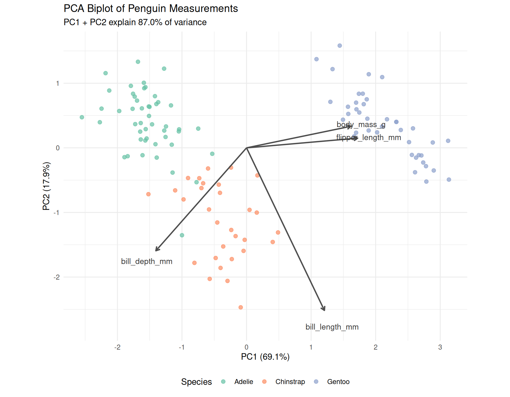
6.5 Interpretation
PCA Interpretation
- PC1 primarily captures overall body size (flipper length and body mass load strongly)
- PC2 captures bill shape (bill length and depth in opposite directions)
- Gentoo penguins separate clearly on PC1 (larger body size)
- Adelie and Chinstrap overlap more but separate on PC2 (bill dimensions)
7 Part 7: Machine Learning with tidymodels
We will build a classification model to predict penguin species from morphological measurements.
7.1 Prepare the modeling data
# Remove rows with missing values for the features we'll use
penguins_ml <- penguins |>
  select(species, bill_length_mm, bill_depth_mm,
         flipper_length_mm, body_mass_g) |>
  drop_na()

# Check class balance
penguins_ml |> count(species)
# A tibble: 3 × 2
species n
<fct> <int>
1 Adelie 48
2 Chinstrap 30
3 Gentoo 40
Understanding data preparation for ML
What it does:
select(...)keeps only the columns we need: the target variable (species) and the four numeric predictors (the measurements).drop_na()removes any rows that have missing values in any of these columns.count(species)shows us how many penguins of each species remain in our dataset.
Why we do it:
Machine learning algorithms cannot handle missing values: they need complete data for every observation. By selecting only the relevant columns first, we avoid accidentally removing rows that have missing values in columns we don’t even use.
Checking the class balance (how many of each species) is important because if one species were much rarer than others, our model might struggle to learn its patterns. In our case, we have roughly similar numbers of each species, which is good.
7.2 Split data into training and testing sets
# for reproducibility
set.seed(42)  # answer to life the universe and everything!

# Create train/test split (75/25)
penguins_split <-
  initial_split(penguins_ml,
                prop = 0.75,
                strata = species)

penguins_train <- training(penguins_split)
penguins_test <- testing(penguins_split)

cat("Training set size:", nrow(penguins_train), "\n")
Training set size: 88 cat("Test set size:", nrow(penguins_test), "\n")Test set size: 30
Understanding train/test splitting
What it does:
set.seed(42)fixes the random number generator so that the “random” split is the same every time we run the code.initial_split(..., prop = 0.75, strata = species)divides the data: 75% for training, 25% for testing. Thestrata = speciesargument ensures that each species is represented proportionally in both sets.training()andtesting()extract the two subsets from the split object.
Why we do it:
Why split the data? We need to evaluate how well our model performs on data it has never seen. If we trained and tested on the same data, the model could simply memorise the answers rather than learning general patterns. This would give us an overly optimistic estimate of performance.
Why set a seed? Data splitting involves randomness. Without a seed, you would get different training and testing sets each time you run the code, making your results impossible to reproduce. Setting a seed ensures that you (and anyone else running your code) get identical results.
Why stratify? Imagine if, by chance, all the Chinstrap penguins ended up in the training set and none in the test set. We couldn’t evaluate how well the model predicts Chinstraps! Stratified sampling prevents this by ensuring each species appears in both sets in the same proportions as the original data.
7.3 Define the model workflow
We’ll use a random forest classifier:
# Define the model specification
rf_spec <- rand_forest(
  trees = 500,
  mtry = 2,
  min_n = 5
) |>
  set_engine("ranger") |>
  set_mode("classification")

# Define the recipe (preprocessing steps)
penguins_recipe <- recipe(species ~ ., data = penguins_train) |>
  step_normalize(all_numeric_predictors())  # scale numeric features

# Combine into a workflow
rf_workflow <- workflow() |>
  add_recipe(penguins_recipe) |>
  add_model(rf_spec)

rf_workflow
══ Workflow ════════════════════════════════════════════════════════════════════
Preprocessor: Recipe
Model: rand_forest()
── Preprocessor ────────────────────────────────────────────────────────────────
1 Recipe Step
• step_normalize()
── Model ───────────────────────────────────────────────────────────────────────
Random Forest Model Specification (classification)
Main Arguments:
mtry = 2
trees = 500
min_n = 5
Computational engine: ranger
Understanding the model specification
What it does:
rand_forest(...)specifies that we want a Random Forest model with particular settings:trees = 500: build 500 individual decision treesmtry = 2: at each split, randomly consider only 2 of the 4 predictorsmin_n = 5: don’t split a node if it has fewer than 5 observations
set_engine("ranger")tells tidymodels to use therangerpackage as the computational backend.set_mode("classification")specifies that we’re predicting categories (species), not continuous numbers.
Why we do it:
Why Random Forest? A Random Forest is an ensemble method: it builds many decision trees and combines their predictions by voting. This makes it robust, accurate, and resistant to overfitting. It works well “out of the box” without much tuning, making it ideal for learning.
Why these parameter values?
trees = 500: More trees generally means better and more stable predictions, at the cost of computation time. 500 is a reasonable default.mtry = 2: By randomly restricting which predictors each tree can consider at each split, we ensure the trees are diverse. If every tree used the same “best” predictor first, they would all be very similar, defeating the purpose of an ensemble. A common rule of thumb for classification issqrt(number of predictors), which for 4 predictors is 2.min_n = 5: This prevents trees from creating very specific rules based on just one or two observations, which would be overfitting.
Why separate specification from fitting? Tidymodels separates what model you want from how to fit it. This modular design lets you easily swap models (try logistic regression instead of random forest) without rewriting the rest of your code.
Understanding the preprocessing recipe
What it does:
recipe(species ~ ., data = penguins_train)declares the modelling task: predictspeciesusing all other columns (.means “everything else”). Thedataargument is used only to identify column names and types (no actual fitting happens yet).step_normalize(all_numeric_predictors())adds a preprocessing step that will centre and scale all numeric predictors to have mean 0 and standard deviation 1.
Why we do it:
Why use a recipe? A recipe is a blueprint for data preprocessing. It records what transformations to apply, but doesn’t apply them yet. This is crucial because:
- The same transformations must be applied identically to training data, test data, and any future data.
- Parameters (like the mean and standard deviation used for scaling) must be learned from the training data only, then applied to test data. If we scaled the test data using its own statistics, we would be “peeking” at test data during training.
Why normalise? While Random Forests don’t strictly require normalisation (they’re based on splitting rules, not distances), it’s good practice and essential for many other algorithms. Including it here means if you later switch to a model that does require scaling (like logistic regression or SVM), your code still works.
Understanding the workflow
What it does:
workflow()creates an empty workflow container.add_recipe(penguins_recipe)attaches the preprocessing recipe.add_model(rf_spec)attaches the model specification.
Why we do it:
A workflow bundles preprocessing and modelling into a single object. This has several advantages:
- Simplicity: You fit the workflow once, and it automatically applies preprocessing then fits the model.
- Safety: It ensures preprocessing parameters are learned from training data and correctly applied to new data.
- Portability: The fitted workflow can be saved and reused, carrying all necessary information with it.
Think of it as packaging your entire analysis pipeline into one neat object.
7.4 Train the model
# Fit the model on training data
rf_fit <- rf_workflow |>
  fit(data = penguins_train)

rf_fit
══ Workflow [trained] ══════════════════════════════════════════════════════════
Preprocessor: Recipe
Model: rand_forest()
── Preprocessor ────────────────────────────────────────────────────────────────
1 Recipe Step
• step_normalize()
── Model ───────────────────────────────────────────────────────────────────────
Ranger result
Call:
ranger::ranger(x = maybe_data_frame(x), y = y, mtry = min_cols(~2, x), num.trees = ~500, min.node.size = min_rows(~5, x), num.threads = 1, verbose = FALSE, seed = sample.int(10^5, 1), probability = TRUE)
Type: Probability estimation
Number of trees: 500
Sample size: 88
Number of independent variables: 4
Mtry: 2
Target node size: 5
Variable importance mode: none
Splitrule: gini
OOB prediction error (Brier s.): 0.01879658
Understanding model training
What it does:
fit(data = penguins_train) executes the workflow on the training data:
- The recipe is “prepped”: it learns the preprocessing parameters (means and standard deviations for normalisation) from the training data.
- The training data is transformed according to the recipe.
- The Random Forest model is trained on the transformed training data.
The result, rf_fit, is a fitted workflow containing both the learned preprocessing parameters and the trained model.
Why we do it:
This is where the actual learning happens. The Random Forest algorithm examines the training data, builds 500 decision trees, and learns rules like “if bill length > 45mm and bill depth < 15mm, this is probably a Gentoo”.
We fit on training data only (the test data remains completely unseen), preserving it as an honest evaluation set.
7.5 Evaluate on test data
# Make predictions on test set
penguins_predictions <- rf_fit |>
  predict(penguins_test) |>
  bind_cols(penguins_test)

# View predictions
penguins_predictions |>
  select(species, .pred_class) |>
  head(10)
# A tibble: 10 × 2
species .pred_class
<fct> <fct>
1 Adelie Adelie
2 Adelie Adelie
3 Adelie Adelie
4 Adelie Adelie
5 Adelie Adelie
6 Adelie Adelie
7 Adelie Adelie
8 Adelie Adelie
9 Adelie Adelie
10 Adelie Adelie
Understanding test set predictions
What it does:
predict(penguins_test)takes the fitted workflow and applies it to the test data:- First, it transforms the test data using the preprocessing recipe (with parameters learned from training data).
- Then, it runs the transformed data through the trained model to get predictions.
- The output is a tibble with a column
.pred_classcontaining the predicted species.
bind_cols(penguins_test)attaches these predictions to the original test data, so we can compare predictions to actual species.
Why we do it:
Now we see how well our model generalises to new data. The test set simulates real-world deployment: the model has never seen these penguins before.
By keeping predictions alongside the true species, we can directly compare them and calculate performance metrics.
7.6 Model performance metrics
# Accuracy
accuracy(penguins_predictions,
         truth = species,
         estimate = .pred_class)
# A tibble: 1 × 3
.metric .estimator .estimate
<chr> <chr> <dbl>
1 accuracy multiclass 1# Confusion matrix
conf_mat(penguins_predictions,
truth = species,
estimate = .pred_class) Truth
Prediction Adelie Chinstrap Gentoo
Adelie 12 0 0
Chinstrap 0 8 0
Gentoo 0 0 10
Understanding accuracy
What it does:
Calculates accuracy: the proportion of predictions that were correct.
\[\text{Accuracy} = \frac{\text{Number of correct predictions}}{\text{Total number of predictions}}\]
Why we do it:
Accuracy is intuitive: it answers “what percentage did we get right?” However, it can be misleading with imbalanced classes. If 90% of penguins were Adelie, a model that always guessed “Adelie” would have 90% accuracy but would be useless for identifying other species.
In our case, classes are roughly balanced, so accuracy is a reasonable metric.
Understanding the confusion matrix
What it does:
Creates a confusion matrix: a table showing, for each actual species, how many were predicted as each species.
            Predicted
Actual      Adelie  Chinstrap  Gentoo
Adelie         12         0       0
Chinstrap       0         8       0
Gentoo          0         0      10
Why we do it:
The confusion matrix reveals where errors occur. Maybe the model confuses Adelie and Chinstrap but never misclassifies Gentoo. This detailed view helps diagnose problems and understand model behaviour beyond a single accuracy number.
- Diagonal entries: correct predictions
- Off-diagonal entries: errors (actual species in row, predicted species in column)
7.7 Visualize the confusion matrix
penguins_predictions |>
  conf_mat(truth = species, estimate = .pred_class) |>
  autoplot(type = "heatmap") +
  scale_fill_gradient(low = "white", high = "steelblue") +
  labs(title = "Confusion Matrix: Random Forest Classification") +
  theme(axis.text.x = element_text(angle = 45, hjust = 1))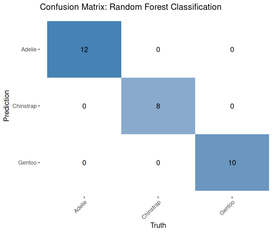
7.8 Cross-validation for robust evaluation
set.seed(2026) # current year :)
# Create 5-fold cross-validation
cv_folds <- vfold_cv(penguins_train, v = 5, strata = species)
# Fit with cross-validation
cv_results <- rf_workflow |>
fit_resamples(
resamples = cv_folds,
metrics = metric_set(accuracy, roc_auc)
)
# Collect metrics
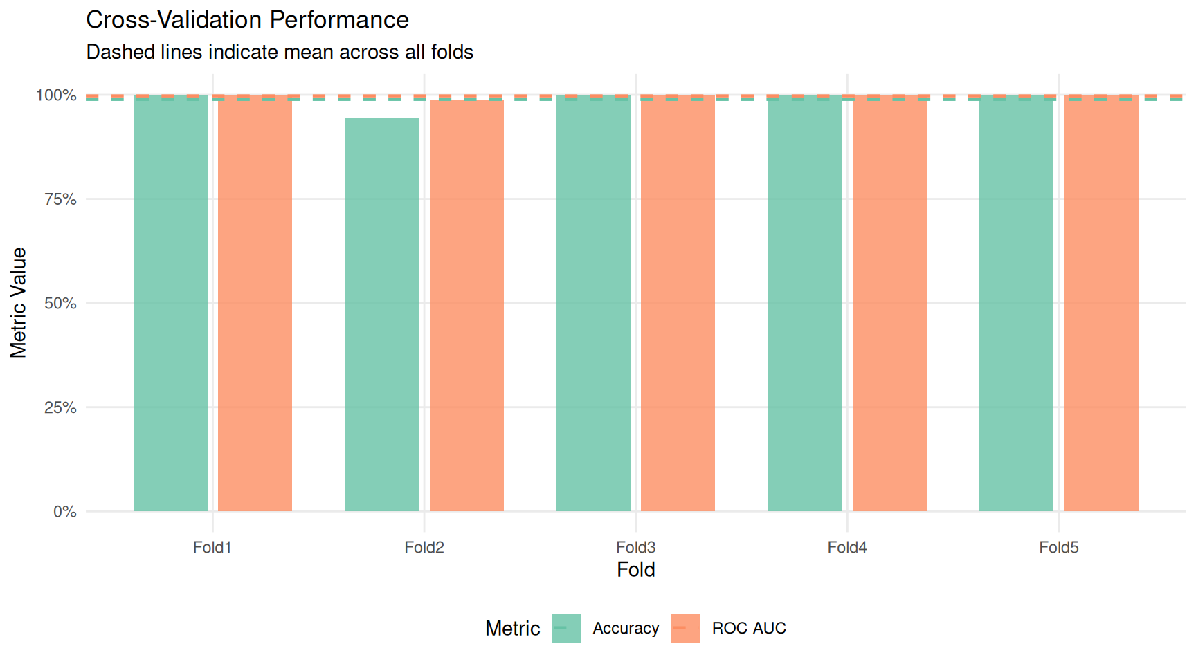
collect_metrics(cv_results)# A tibble: 2 × 6
.metric .estimator mean n std_err .config
<chr> <chr> <dbl> <int> <dbl> <chr>
1 accuracy multiclass 0.989 5 0.0111 pre0_mod0_post0
2 roc_auc hand_till 0.997 5 0.00270 pre0_mod0_post0
Understanding cross-validation
What it does:
set.seed(2026)ensures reproducible fold assignments.vfold_cv(penguins_train, v = 5, strata = species)divides the training data into 5 equal parts (folds), stratified by species.fit_resamples(...)performs 5-fold cross-validation:- Iteration 1: train on folds 2–5, evaluate on fold 1
- Iteration 2: train on folds 1, 3–5, evaluate on fold 2
- … and so on
metrics = metric_set(accuracy, roc_auc)specifies which metrics to calculate.collect_metrics(cv_results)summarises the results, showing the mean and standard error of each metric across the 5 folds.
Why we do it:
Why cross-validate? A single train/test split gives us one estimate of model performance. But what if we got lucky (or unlucky) with that particular split? Cross-validation provides multiple estimates, letting us assess how stable our performance is.
How to interpret the results:
- Mean accuracy: the average accuracy across all 5 folds (a more reliable estimate than a single split).
- Standard error: indicates how much the accuracy varied between folds. A small standard error means consistent performance; a large one suggests the model’s performance depends heavily on which data it sees.
What is ROC AUC? The Area Under the Receiver Operating Characteristic curve measures how well the model distinguishes between classes across all possible decision thresholds. Values range from 0.5 (random guessing) to 1.0 (perfect separation). It’s particularly useful when you care about ranking predictions, not just the final class labels.
# Extract per-fold metrics
cv_fold_metrics <- cv_results |>
  collect_metrics(summarize = FALSE)

# Create a summary for plotting
cv_summary <- cv_results |>
  collect_metrics()

# Plot metrics across folds
ggplot(cv_fold_metrics, aes(x = id, y = .estimate, fill = .metric)) +
  geom_col(position = position_dodge(width = 0.8), width = 0.7, alpha = 0.8) +
  geom_hline(
    data = cv_summary,
    aes(yintercept = mean, color = .metric),
    linetype = "dashed",
    linewidth = 0.8
  ) +
  scale_fill_brewer(palette = "Set2", labels = c("Accuracy", "ROC AUC")) +
  scale_color_brewer(palette = "Set2", labels = c("Accuracy", "ROC AUC")) +
  scale_y_continuous(limits = c(0, 1), labels = scales::percent) +
  labs(
    title = "Cross-Validation Performance",
    subtitle = "Dashed lines indicate mean across all folds",
    x = "Fold",
    y = "Metric Value",
    fill = "Metric",
    color = "Metric"
  ) +
  theme_minimal() +
  theme(
    legend.position = "bottom",
    panel.grid.minor = element_blank()
  )
cv_fold_metrics |>
  mutate(.metric = case_when(
    .metric == "accuracy" ~ "Accuracy",
    .metric == "roc_auc" ~ "ROC AUC"
  )) |>
  ggplot(aes(x = id, y = .estimate, color = .metric)) +
  geom_segment(
    aes(xend = id, yend = 0.8),
    linewidth = 1,
    position = position_dodge(width = 0.4)
  ) +
  geom_point(size = 4, position = position_dodge(width = 0.4)) +
  scale_color_brewer(palette = "Set2") +
  scale_y_continuous(limits = c(0.8, 1), labels = scales::percent) +
  labs(
    title = "Cross-Validation Performance",
    x = "Fold",
    y = "Metric Value",
    color = "Metric"
  ) +
  theme_minimal() +
  theme(legend.position = "bottom")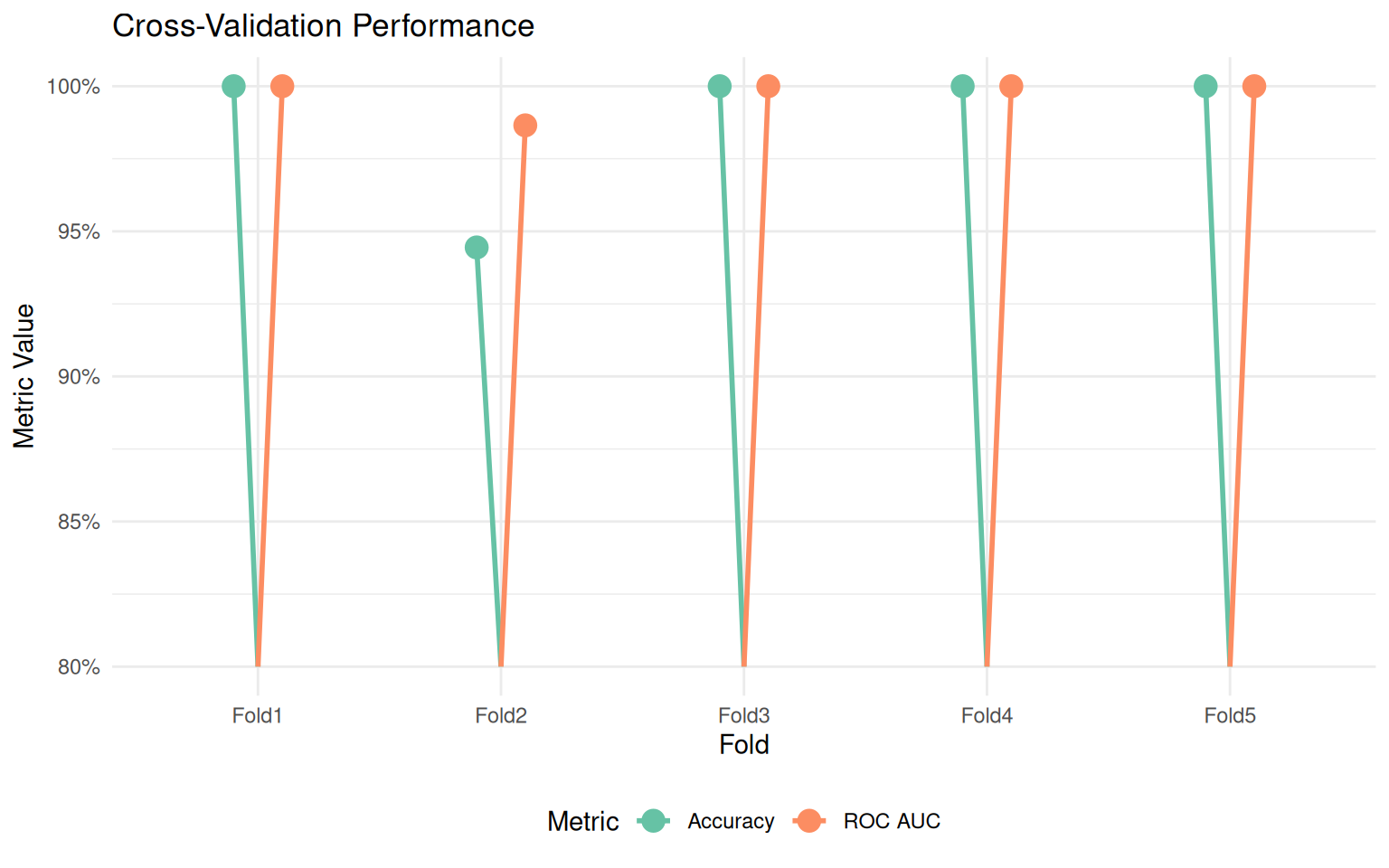
cv_fold_metrics |>
  mutate(.metric = case_when(
    .metric == "accuracy" ~ "Accuracy",
    .metric == "roc_auc" ~ "ROC AUC"
  )) |>
  ggplot(aes(x = .metric, y = .estimate)) +
  geom_jitter(width = 0.1, size = 3, alpha = 0.6, color = "skyblue2") +
  stat_summary(
    fun = mean,
    geom = "crossbar",
    width = 0.5,
    color = "coral2",
    linewidth = 0.5
  ) +
  scale_y_continuous(limits = c(0.8, 1.1), labels = scales::percent) +
  labs(
    title = "Cross-Validation Performance",
    subtitle = "Individual folds with mean (red line)",
    x = NULL,
    y = "Metric Value"
  ) +
  theme_minimal()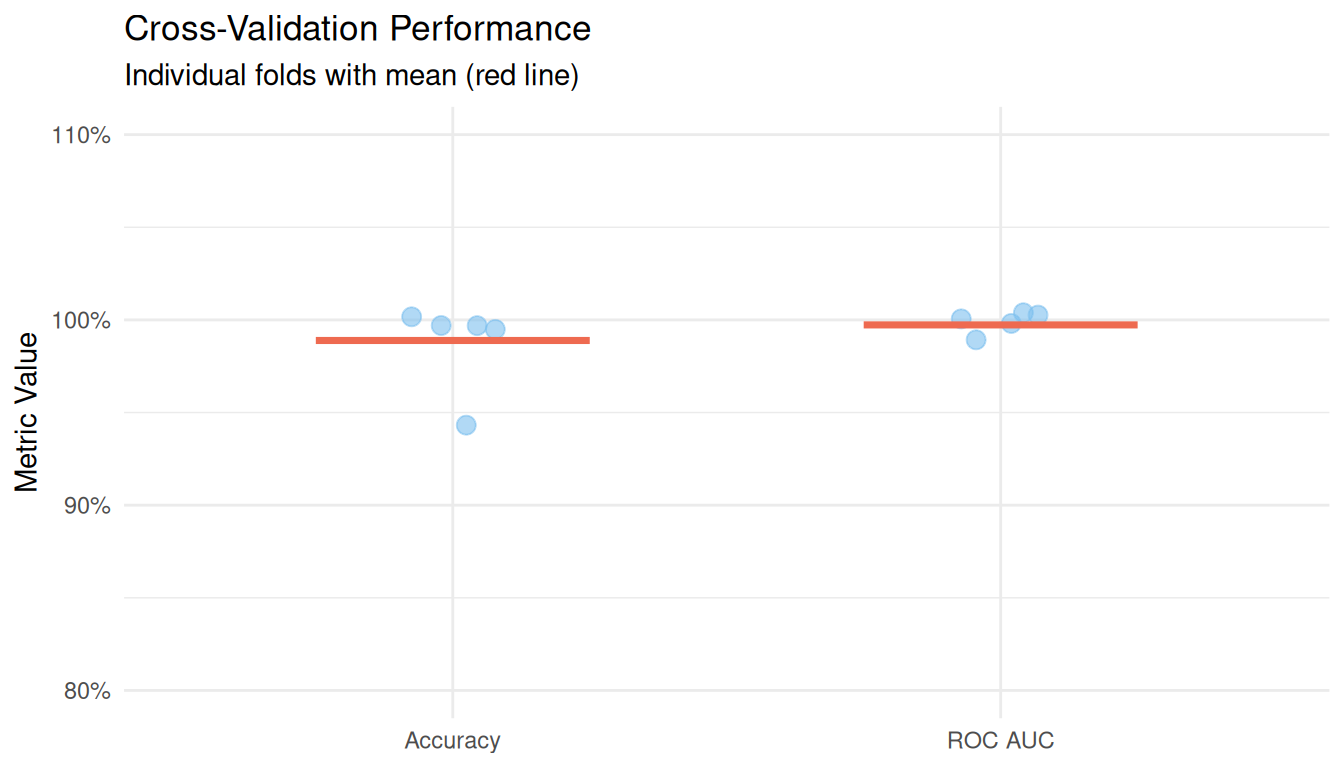
cv_fold_metrics |>
  mutate(.metric = case_when(
    .metric == "accuracy" ~ "Accuracy",
    .metric == "roc_auc" ~ "ROC AUC"
  )) |>
  ggplot(aes(x = id, y = .estimate, color = .metric, group = .metric)) +
  geom_line(linewidth = 1) +
  geom_point(size = 3) +
  scale_color_brewer(palette = "Set2") +
  scale_y_continuous(limits = c(0.8, 1), labels = scales::percent) +
  labs(
    title = "Cross-Validation Performance Across Folds",
    x = "Fold",
    y = "Metric Value",
    color = "Metric"
  ) +
  theme_minimal() +
  theme(legend.position = "bottom")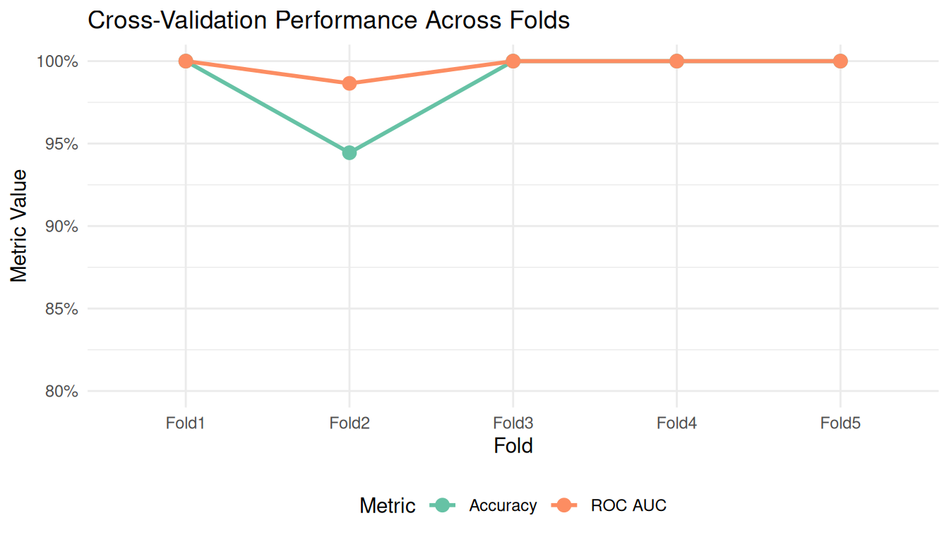
The Complete ML Workflow
Here’s the full machine learning workflow in context:
Prepare data: Select relevant columns, remove missing values.
Split data: Separate into training (for learning) and testing (for evaluation).
Define the model: Specify what algorithm to use and its parameters.
Create a recipe: Define preprocessing steps (like normalisation).
Build a workflow: Combine recipe and model into one object.
Train: Fit the workflow on training data.
Predict: Apply the trained workflow to test data.
Evaluate: Calculate metrics to assess performance.
Cross-validate: Get robust performance estimates with uncertainty.
This workflow, enabled by the tidymodels framework, is modular and reproducible. You can easily substitute different models, add preprocessing steps, or change evaluation metrics, all while maintaining the same overall structure.
Glossary of Key ML Terms
| Term | Definition |
|---|---|
| Classification | Predicting which category an observation belongs to |
| Training set | Data used to fit the model |
| Test set | Data held out to evaluate model performance |
| Overfitting | When a model memorises training data but fails on new data |
| Random Forest | An ensemble of decision trees that vote on predictions |
| Recipe | A blueprint for preprocessing steps |
| Workflow | A container bundling preprocessing and modelling |
| Cross-validation | Repeated train/test splits for robust evaluation |
| Accuracy | Proportion of correct predictions |
| Confusion matrix | Table showing prediction errors by class |
| ROC AUC | Metric measuring class separation quality |
8 Using the Classifier with New Data
Once we have a trained model, the real value comes from using it to classify new observations. This section shows how to predict the species of penguins based on their measurements.
8.1 Predicting a single observation
To classify a new penguin, we create a data frame with the same columns used for training, then pass it to the predict() function:
# Create a new observation
new_penguin <- tibble(

  bill_length_mm = 45.0,
  bill_depth_mm = 15.0,
  flipper_length_mm = 215,
  body_mass_g = 5000
)

# Predict the species
predict(rf_fit, new_penguin)
# A tibble: 1 × 1
.pred_class
<fct>
1 Gentoo 8.2 Getting prediction probabilities
Often we want to know not just the predicted class, but how confident the model is. We can request class probabilities:
# Get prediction probabilities for each species
predict(rf_fit, new_penguin, type = "prob")
# A tibble: 1 × 3
.pred_Adelie .pred_Chinstrap .pred_Gentoo
<dbl> <dbl> <dbl>
1 0 0.0004 1.000We can combine the predicted class with probabilities for a complete picture:
# Combine class prediction with probabilities
new_penguin |>
  bind_cols(predict(rf_fit, new_penguin)) |>
  bind_cols(predict(rf_fit, new_penguin, type = "prob"))
# A tibble: 1 × 8
bill_length_mm bill_depth_mm flipper_length_mm body_mass_g .pred_class
<dbl> <dbl> <dbl> <dbl> <fct>
1 45 15 215 5000 Gentoo
# ℹ 3 more variables: .pred_Adelie <dbl>, .pred_Chinstrap <dbl>,
# .pred_Gentoo <dbl>8.3 Predicting multiple observations
The same approach works for multiple penguins at once:
# Create several new observations
new_penguins <- tibble(
  bill_length_mm = c(39.0, 48.5, 52.0),
  bill_depth_mm = c(18.5, 14.0, 19.0),
  flipper_length_mm = c(185, 220, 195),
  body_mass_g = c(3600, 5400, 3800)
)

# Predict all at once
new_penguins |>
  bind_cols(predict(rf_fit, new_penguins)) |>
  bind_cols(predict(rf_fit, new_penguins, type = "prob")) |>
  mutate(across(where(is.numeric) & starts_with(".pred_"), ~ round(., 3)))
# A tibble: 3 × 8
bill_length_mm bill_depth_mm flipper_length_mm body_mass_g .pred_class
<dbl> <dbl> <dbl> <dbl> <fct>
1 39 18.5 185 3600 Adelie
2 48.5 14 220 5400 Gentoo
3 52 19 195 3800 Chinstrap
# ℹ 3 more variables: .pred_Adelie <dbl>, .pred_Chinstrap <dbl>,
# .pred_Gentoo <dbl>8.4 A helper function for classification
For convenience, we can wrap the prediction logic into a reusable function:
classify_penguin <- function(bill_length, bill_depth, flipper_length, body_mass,
                             model = rf_fit) {

 # Create the input data frame (works with single values or vectors)
  new_data <- tibble(
    bill_length_mm = bill_length,
    bill_depth_mm = bill_depth,
    flipper_length_mm = flipper_length,
    body_mass_g = body_mass
  )

  # Get predictions
  predictions <- new_data |>
    bind_cols(predict(model, new_data)) |>
    bind_cols(predict(model, new_data, type = "prob")) |>
    rename(predicted_species = .pred_class) |>
    mutate(across(where(is.numeric) & starts_with(".pred_"), ~ round(., 3)))

  return(predictions)
}
Now we can classify penguins with a simple function call:
# Single penguin
classify_penguin(
  bill_length = 38.5,
  bill_depth = 18.0,
  flipper_length = 190,
  body_mass = 3500
)
# A tibble: 1 × 8
bill_length_mm bill_depth_mm flipper_length_mm body_mass_g predicted_species
<dbl> <dbl> <dbl> <dbl> <fct>
1 38.5 18 190 3500 Adelie
# ℹ 3 more variables: .pred_Adelie <dbl>, .pred_Chinstrap <dbl>,
# .pred_Gentoo <dbl># Multiple penguins using vectors
classify_penguin(
bill_length = c(38.5, 47.0, 49.0),
bill_depth = c(18.0, 14.5, 18.5),
flipper_length = c(190, 215, 195),
body_mass = c(3500, 5200, 3700)
)# A tibble: 3 × 8
bill_length_mm bill_depth_mm flipper_length_mm body_mass_g predicted_species
<dbl> <dbl> <dbl> <dbl> <fct>
1 38.5 18 190 3500 Adelie
2 47 14.5 215 5200 Gentoo
3 49 18.5 195 3700 Chinstrap
# ℹ 3 more variables: .pred_Adelie <dbl>, .pred_Chinstrap <dbl>,
# .pred_Gentoo <dbl>8.5 Visualising prediction confidence
We can visualise the prediction probabilities to better understand model confidence:
# Define test cases
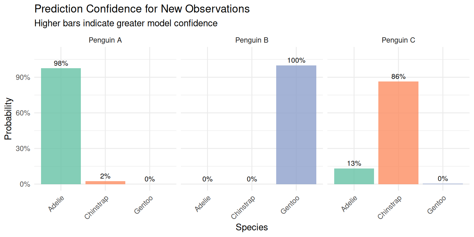
test_ids <- c("Penguin A", "Penguin B", "Penguin C")
bill_lengths <- c(38.5, 47.0, 45.0)
bill_depths <- c(18.0, 14.5, 17.0)
flipper_lengths <- c(190, 215, 200)
body_masses <- c(3500, 5200, 4000)
# Get predictions using the classify function
test_predictions <- classify_penguin(
bill_length = bill_lengths,
bill_depth = bill_depths,
flipper_length = flipper_lengths,
body_mass = body_masses
) |>
mutate(id = test_ids, .before = 1)
# Reshape for plotting
test_predictions |>
select(id, predicted_species, starts_with(".pred_")) |>
pivot_longer(
cols = c(.pred_Adelie, .pred_Chinstrap, .pred_Gentoo),
names_to = "species",
values_to = "probability",
names_prefix = ".pred_"
) |>
ggplot(aes(x = species, y = probability, fill = species)) +
geom_col(alpha = 0.8) +
geom_text(aes(label = scales::percent(probability, accuracy = 1)),
vjust = -0.5, size = 3) +
facet_wrap(~ id) +
scale_fill_brewer(palette = "Set2") +
scale_y_continuous(limits = c(0, 1.1), labels = scales::percent) +
labs(
title = "Prediction Confidence for New Observations",
subtitle = "Higher bars indicate greater model confidence",
x = "Species",
y = "Probability"
) +
theme_minimal() +
theme(
legend.position = "none",
axis.text.x = element_text(angle = 45, hjust = 1)
)
9 Summary and Conclusions
In this mini-project, you practiced the complete workflow of reproducible data analysis:
Project organization: Created a logical folder structure separating raw data, processed data, scripts, and outputs.
Data import: Read messy data with explicit parameters, handling multiple representations of missing values.
Data cleaning: Applied systematic cleaning steps using tidyverse functions, documenting each transformation.
Exploratory analysis: Computed descriptive statistics and identified patterns in the data.
Visualization: Created informative plots following the grammar of graphics.
Dimensionality reduction: Applied PCA to understand the multivariate structure of the data.
Machine learning: Built and evaluated a classification model using the tidymodels framework.
Best Practices Learned
- Always keep raw data unmodified
- Document every data transformation
- Use consistent naming conventions
- Set random seeds for reproducibility
- Validate data at each step
- Split data before any model training
- Use cross-validation for robust estimates
10 Exercises
Try these extensions to deepen your understanding:
Data cleaning: What other data quality issues might exist? How would you handle outliers?
Visualization: Create a plot showing the relationship between flipper length and body mass, with separate panels for each island.
PCA: Re-run PCA on each species separately. How do the loadings differ?
Machine learning: Try a different model (logistic regression, decision tree) and compare performance. Which features are most important?
Reproducibility: Create a separate R script that runs the entire analysis from raw data to final model, with no manual intervention required.
11 Session Info
For reproducibility, always record the versions of R and packages used:
sessionInfo()R version 4.5.0 (2025-04-11)
Platform: x86_64-pc-linux-gnu
Running under: Ubuntu 24.04.4 LTS
Matrix products: default
BLAS: /usr/lib/x86_64-linux-gnu/blas/libblas.so.3.12.0
LAPACK: /usr/lib/x86_64-linux-gnu/lapack/liblapack.so.3.12.0 LAPACK version 3.12.0
locale:
[1] LC_CTYPE=en_US.UTF-8 LC_NUMERIC=C
[3] LC_TIME=en_US.UTF-8 LC_COLLATE=en_US.UTF-8
[5] LC_MONETARY=en_US.UTF-8 LC_MESSAGES=en_US.UTF-8
[7] LC_PAPER=en_US.UTF-8 LC_NAME=C
[9] LC_ADDRESS=C LC_TELEPHONE=C
[11] LC_MEASUREMENT=en_US.UTF-8 LC_IDENTIFICATION=C
time zone: Europe/Lisbon
tzcode source: system (glibc)
attached base packages:
[1] stats graphics grDevices utils datasets methods base
other attached packages:
[1] yardstick_1.3.2 workflowsets_1.1.1 workflows_1.3.0 tune_2.0.1
[5] tailor_0.1.0 rsample_1.3.2 recipes_1.3.1 parsnip_1.4.1
[9] modeldata_1.5.1 infer_1.1.0 dials_1.4.2 scales_1.4.0
[13] broom_1.0.12 tidymodels_1.4.1 GGally_2.2.1 corrplot_0.95
[17] skimr_2.2.2 janitor_2.2.1 lubridate_1.9.4 forcats_1.0.0
[21] stringr_1.6.0 dplyr_1.2.1 purrr_1.2.2 readr_2.1.5
[25] tidyr_1.3.2 tibble_3.3.1 ggplot2_4.0.2 tidyverse_2.0.0
loaded via a namespace (and not attached):
[1] tidyselect_1.2.1 timeDate_4052.112 farver_2.1.2
[4] S7_0.2.0 fastmap_1.2.0 digest_0.6.37
[7] rpart_4.1.24 timechange_0.3.0 lifecycle_1.0.5
[10] survival_3.8-3 magrittr_2.0.4 compiler_4.5.0
[13] rlang_1.2.0 tools_4.5.0 utf8_1.2.6
[16] yaml_2.3.10 data.table_1.17.2 knitr_1.50
[19] labeling_0.4.3 htmlwidgets_1.6.4 bit_4.6.0
[22] plyr_1.8.9 DiceDesign_1.10 repr_1.1.7
[25] RColorBrewer_1.1-3 withr_3.0.2 nnet_7.3-20
[28] grid_4.5.0 sparsevctrs_0.3.6 future_1.70.0
[31] globals_0.19.1 MASS_7.3-65 cli_3.6.6
[34] crayon_1.5.3 rmarkdown_2.29 generics_0.1.4
[37] rstudioapi_0.17.1 future.apply_1.20.2 tzdb_0.5.0
[40] splines_4.5.0 parallel_4.5.0 base64enc_0.1-3
[43] vctrs_0.7.1 hardhat_1.4.2 Matrix_1.7-3
[46] jsonlite_2.0.0 hms_1.1.3 bit64_4.6.0-1
[49] listenv_0.10.1 gower_1.0.2 glue_1.8.0
[52] parallelly_1.46.1 ggstats_0.9.0 codetools_0.2-20
[55] stringi_1.8.7 gtable_0.3.6 GPfit_1.0-9
[58] pillar_1.11.1 furrr_0.4.0 htmltools_0.5.8.1
[61] ipred_0.9-15 lava_1.8.2 R6_2.6.1
[64] lhs_1.2.1 vroom_1.6.5 evaluate_1.0.5
[67] lattice_0.22-7 backports_1.5.0 snakecase_0.11.1
[70] class_7.3-23 Rcpp_1.0.14 nlme_3.1-168
[73] prodlim_2026.03.11 ranger_0.18.0 mgcv_1.9-3
[76] xfun_0.52 pkgconfig_2.0.3