3. The role of public databases
A few bioinformatics centres of excellence worldwide are responsible for collecting, organising, and providing open access to published biological data. Key centres include:
This work began in the early 1980s, when DNA sequence data started to accumulate in scientific publications. To manage this, the ENA - European Nucleotide Archive) was created, as well as the GenBank at NCBI, and DDBJ at NIG.
Who owns the data? From the start, the bioinformatics community has promoted open data sharing and made it a reality through international collaborations, for example:
This openness has allowed researchers to fully benefit from large-scale projects such as the Human Genome Project and The Encyclopedia of DNA Elements (ENCODE). Importantly, open sharing is not limited to big collaborations. Increasingly, funding policies reflect the principle that if research is publicly funded, the resulting data should also be made publicly accessible for others to use.
4. Making data useful
Open access is only the first step. For data to be truly useful, it must also be recorded and organised in a way that supports consistent interpretation and reuse. This is where the distinction between primary and secondary databases becomes important.
4.1 Primary vs Secondary databases
Primary databases in bioinformatics are repositories that store raw, unprocessed biological data generated directly from experimental methods, such as nucleotide sequences, protein sequences, and macromolecular structures. Once given a database accession number, the data in primary databases are never changed: they form part of the scientific record.
Secondary databases comprise data derived from the results of analysing primary data. They provide curated, processed, or interpreted data that is derived from the combination of diverse sources of primary data, offering functional insights and higher-level biological context, to derive new knowledge from the public record of science. Secondary databases have become the molecular biologist’s reference library, offering extensive information on nearly every studied gene or gene product. Although often overwhelming, these resources hold enormous potential for discovery through data mining.
4.2 Primary databases
- Store original and unprocessed data from experiments.
- Examples: ENA (European Nucleotide Archive), GenBank (nucleotide sequences), Protein Data Bank (PDB) (3D protein structures), ArrayExpress (gene expression).
- Data is archival and serves as the scientific record, maintaining the integrity of experimental data.
4.3 Secondary databases
- Contain information derived by analyzing, annotating, and curating data from primary databases.
- Examples: InterPro (protein families, integrative protein data), UniProt (protein sequences and functional information).
- Data includes interpretations, predictions, and functional annotations which enrich biological context and usability for researchers.
4.4 Comparison table
| Data |
Raw, experimental |
Processed, curated, interpreted |
| Source |
Direct experiment/researcher input |
Analysis of primary database data |
| Examples |
ENA, GenBank and DDBJ (nucleotide sequence); ArrayExpress and GEO (functional genomics data); PDB (3D macromolecular structures) |
UniProt (sequence and functional information on proteins); Ensembl (variation, function, regulation and more layered onto whole genome sequences); InterPro (protein families, motifs and domains) |
| Function |
Archival record |
Adds annotations and context |
| Modification |
Data not altered |
Data is analyzed, can be modified |
These two types of databases are fundamental to bioinformatics, working together to organize, preserve, and interpret biological data for research and discovery.
4.5 Hybrid databases
Some databases combine both primary and secondary features. For example, UniProt holds experimental peptide sequences but also infers sequences and adds extensive automated (TrEMBL) and manual (SwissProt) annotations. Others separate the two functions into different branches, such as ArrayExpress (raw functional genomics data) and the Expression Atlas (derived expression patterns).
4.6 Molecular databases per data type
Bioinformatics spans many different types of biological data, each with its own uses:
- Genomic data: DNA sequences, variants, and structural alterations.
- Transcriptomic data: RNA expression and splicing patterns.
- Proteomic data: protein expression, modifications, and interactions.
- Metabolomic data: metabolites and metabolic pathways.
- Structural data: 3D structures of proteins and other macromolecules.
- Phenotypic and clinical data: patient traits, disease states, and treatment outcomes.
Together, these diverse datasets provide complementary perspectives and, when integrated, can generate powerful insights into biology and disease.
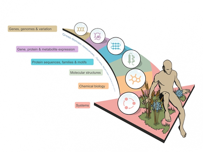
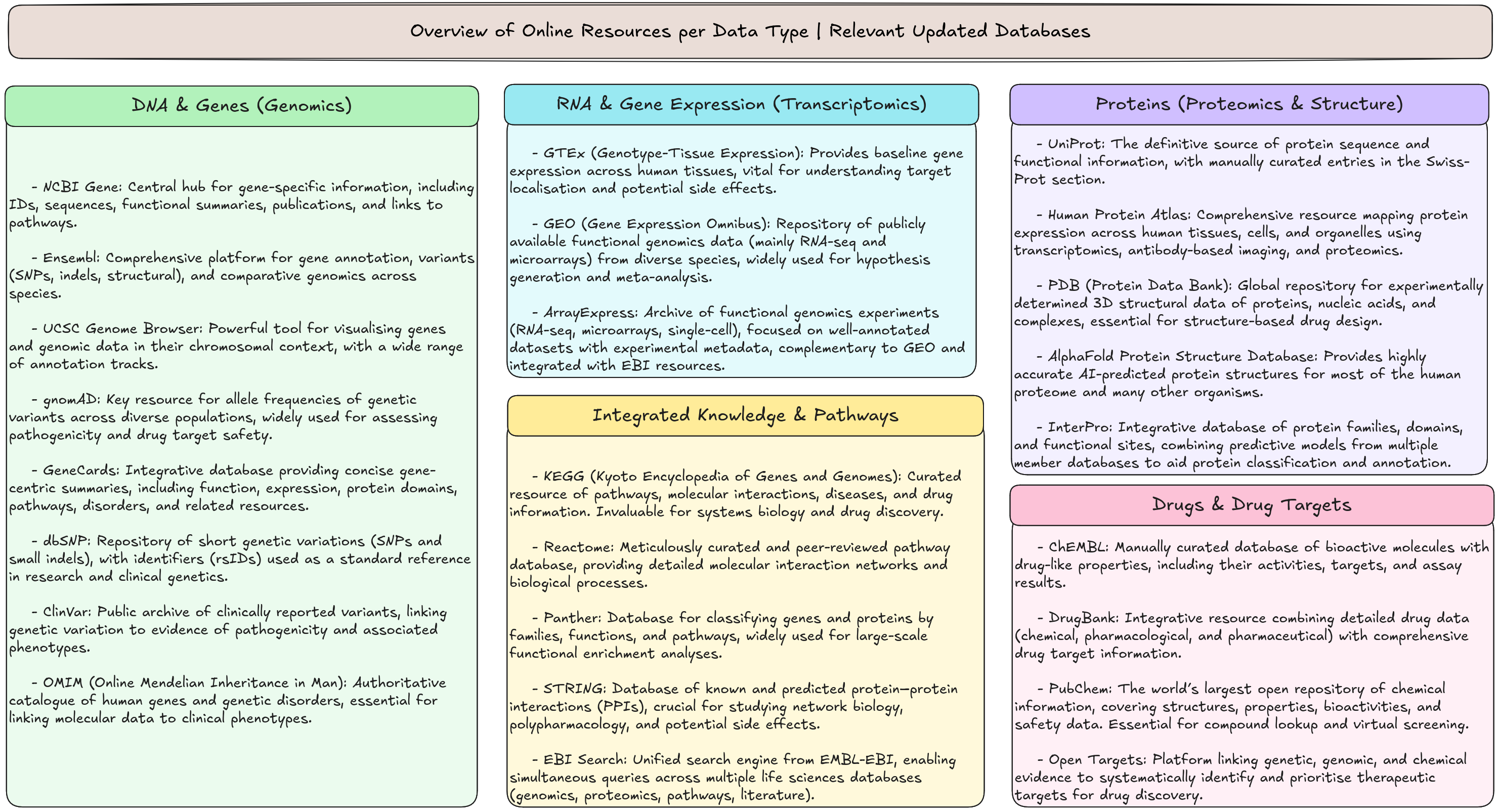
Figure 2 shows an overview of molecular biology data resources: genomic (DNA & genes), transcriptomic (RNA expression), proteomic (proteins & structures), pathway/integrated knowledge, and chemical/drug databases, highlighting the some of the main open-access repositories that support research and drug discovery.
Activity 1: From Data to Databases: Using Dice to Illustrate Principles of Bioinformatics
Duration: ~1.5 hours
Learning goals:
- Experience generating raw data from simple systems (dice).
- Understand the importance of consistent data recording and organization.
- Appreciate how analysis depends on well-structured data.
- Connect classroom activities to bioinformatics databases.
Materials:
- Dice (D4, D6, D8, D10, D12, and D20): one per group (1 or 2 students).
- Paper sheets for data recording.
- Worksheets or laptops.
Activity overview
In this activity we will create a class dataset using dice. Along the way, you will recognize:
- Why standardisation of data is essential to make data usable.
- How sample size affects confidence in results, hence the importance of combining datasets.
- What tidy data means.
- How different dice (D4, D6, D8, D10, D12, D20) relate to variables with different possible measurements.
- The difference between single-variable and multivariate analysis.
Step 1. Roll (15 min)
- Each group is assigned one die.
- Roll it 10 times.
- Record your results in any format you like.
Hint: Record the data in the way that you find most useful and understandable.
Step 2. Compare & Standardise (15 min)
- Join all groups with the same die type (all D4 groups, all D6 groups…).
- Compare how different groups recorded their results.
- Notice differences and discuss the pros and cons of alternative recordings.
- Agree on one standard format.
Lesson: Bioinformatics databases using a standardized data format to allow the pooling together of data from different experiments.
Step 3. Combine (15 min)
- All groups with the same die pool their results.
- Example: one group’s 10 rolls of a D6 = limited evidence, but 50 rolls across all groups = strong evidence about probabilities.
Lesson: Larger sample size = greater confidence in conclusions.
Step 4. Make it Tidy (15)
- Does the agreed upon record standard follow the tidy rule?
- Each variable = a column
- Each observation = a row
- Each value = a cell
Lesson: This is the principle behind how most bioinformatics databases are structured.
Step 5. Reflect on Variables (10 min)
- Different dice = different numbers of possible outcomes.
- D4 = 4 outcomes
- D20 = 20 outcomes
Lesson: Biology is similar:
- Some variables have few states (genotype with 3 possible states).
- Others are more complex (gene expression with many possible values).
Step 6. Single vs. Multivariate Analysis (10 min)
- Single variable: Analyse only one column (e.g. “What is the most common result for D6?”).
- Multivariate: Combine columns (e.g. “When D6 is high, is D20 also high?”).
Lesson: Bioinformatics often moves from univariate summaries (each gene/protein separately) to multivariate models (how variables interact).
Step 7. Wrap-up Reflection (5 min)
Questions:
- What was hardest: generating, recording, or analysing?
- How does this compare to working with real biological data?
- Why do we need curated bioinformatics databases?
Take home message
By rolling dice:
- you’ve built a mini database;
- experienced the challenge of standardisation;
- explored sample size effects;
- practised tidy data;
- understood variable ranges; and
- compared single vs. multivariate analysis.
By the end of this practical class, you should know:
- What made it possible to build a class database?
- Why combine results?
- Sample size = confidence.
- Why tidy format?
- What do different dice represent?
- Different measurement complexities (possible outcomes).
- What’s the difference between single and multivariate analysis?
- One variable vs. relationships between variables.